Data modeling - ANN

An artificial neural network is a nonlinear statistical model composed of interconnected computational units called neurons, arranged in layers. Each neuron computes a weighted combination of its inputs, adds a bias term, and applies a nonlinear activation function. By composing many such transformations, neural networks can represent highly complex functions.

At a mathematical level, an ANN is a parameterized function \(f_\theta: \mathcal X \to \mathcal Y\), where \(\theta\) denotes all trainable weights and biases. The input space \(\mathcal X\) may contain vectors, images, sequences, graphs, or other structured objects. The output space \(\mathcal Y\) may be continuous for regression, categorical for classification, or structured for more complex prediction tasks.

The central learning problem is to choose parameter \(\theta\) that minimize a loss function over observed data:

\[ \hat \theta = \arg\min_\theta \frac{1}{n}\sum_{i=1}^n \mathcal L(y_i, f_\theta(x_i)) \]

The strength of neural networks is that they can learn internal representations of data. In image recognition, early layers may learn edges, middle layers learn the shapes of or textures, and deeper layers can learn object parts. In language modeling, early representations can encode token-level information, while deeper layers encode syntactic, semantic, or contextual relationships. Thus, a neural network can be considered as a representation-learning machine.

1. Historical and Conceptual Background

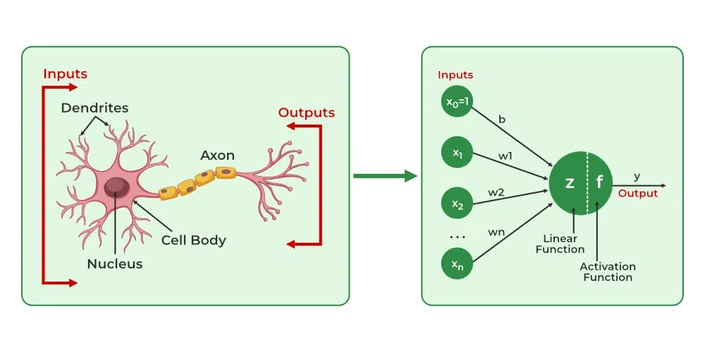
Artificial neural networks are inspired by biological nervous systems. Early neural network ideas can be traced to perceptrons, but the modern revival of neural networks was strongly influence by the development of backpropagation as an efficient algorithm for computing gradients in multilayer networks. Rumelhart, Hinton, and Williams showed how backpropagation could adjust weights in networks of neuron-like units by propagating error derivatives backward through the network1.

Artificial neural networks are inspired by biological nervous systems

Later, universal approximation results showed that sufficiently large feedforward neural networks with appropriate nonlinear activation functions can approximate broad classes of continuous functions on compact sets. Cybenko, for example, proved a universal approximation theorem for networks with a single hidden layer and sigmoidal activation functions2.

In contemporary machine learning, deep learning refers to neural networks with many layers. These networks became especially powerful because of larger datasets, improved optimization methods, specialized hardware, better activation functions, regularization methods, and architectural innovations such as convolution, recurrence, attention, and generative adversarial training, which later on will be discussed.

2. The Basic Neuron

2.1. The Artificial Neuron

NoteDefinition: Artificial Neuron

Let \(x=(x_1, x_2, \dots, x_d)^\top\in \mathbb {R}^d\) be an input vector. An artificial neuron computes

\[ z = w^\top x+ b, \]

where \(w=(w_1, w_2,\dots, w_d)^\top \in \mathbb R^d\) is a weight vector and \(b\in \mathbb R\) is a bias term. The neuron output is:

\[ \alpha = \sigma(z) = \sigma(w^\top x+b), \]

where \(\sigma:\mathbb R\to\mathbb R\) is an activation function.

The neuron therefore performs two operations:

  1. Affine transformation: \(z=w^\top x+ b\).
  2. Nonlinear activation: \(\alpha = \sigma(z)\).

Without the nonlinear activation function, a multilayer network would collapse into a single linear model.

2.2. Why Nonlinearity Is Necessary

Suppose a two-layer network has no nonlinear activation. Then

\[ h = W^{(1)}x + b^{(1)}, \qquad \hat y =W^{(2)}h+ b^{(2)}. \]

Substitute the first equation into the second:

\[ \hat y = W^{(2)}(W^{(1)}x+ b^{(1)}) +b^{(2)}=W^{(2)}W^{(1)}x + W^{(2)}b^{(1)}+b^{(2)}=\tilde{W} x+ \tilde b. \]

Thus, without nonlinear activation functions, stacking layers does not increase expressive power. A deep linear network is still a linear model.

2.3. Activation Functions

Activation functions determine how each neuron transforms its pre-activation value \(z\). They are crucial for approximation power, optimization behavior, and gradient flow.

2.3.1. Sigmoid Function

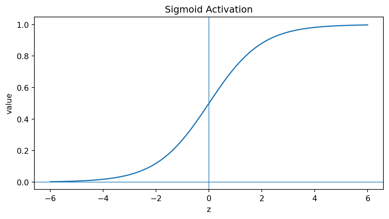
The sigmoid activation is

\[ \sigma(z) = \frac{1}{1+e^{-z}} \]

It maps real numbers to the interval \((0,1)\).

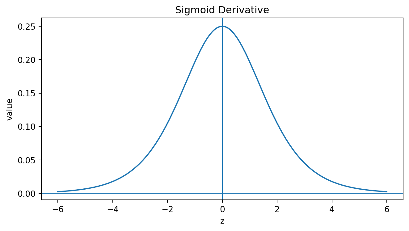
Its derivative is

\[ \sigma' = \sigma(z) (1-\sigma (z)) \]

Let \(\sigma = \frac{1}{1+e^{-z}}\). Then

\[ \sigma' = \frac{e^{-z}}{(1+e^{-z})^2} \] Now observe that

\[ 1- \sigma(z) = 1- \frac{1}{1+e^{-z}}=\frac{e^{-z}}{1+e^{-z}} \]

Therefore,

\[ \sigma(z) (1-\sigma(z))=\frac{1}{1+e^{-z}} \times \frac{e^{-z}}{1+e^{-z}}=\frac{e^{-z}}{(1+e^{-z})^2} =\sigma' \]

The sigmoid is often used in binary classification output layers because it can represent a probability:

\[ \hat p = P(Y=1\,|\,x) = \sigma(z) \]

However, sigmoid units can suffer from gradient saturation when \(|z|\) is large, because the derivative becomes close to zero.

Show code
import numpy as np
import matplotlib.pyplot as plt

z = np.linspace(-6, 6, 500)

sigmoid = 1 / (1 + np.exp(-z))
sigmoid_deriv = sigmoid * (1 - sigmoid)

for y, title in [
    (sigmoid, "Sigmoid Activation"),
    (sigmoid_deriv, "Sigmoid Derivative"),
]:
    plt.figure(figsize=(7, 4))
    plt.plot(z, y)
    plt.axhline(0, linewidth=0.8)
    plt.axvline(0, linewidth=0.8)
    plt.title(title)
    plt.xlabel("z")
    plt.ylabel("value")
    plt.tight_layout()
    plt.show()

2.3.2. Hyperbolic Tangent

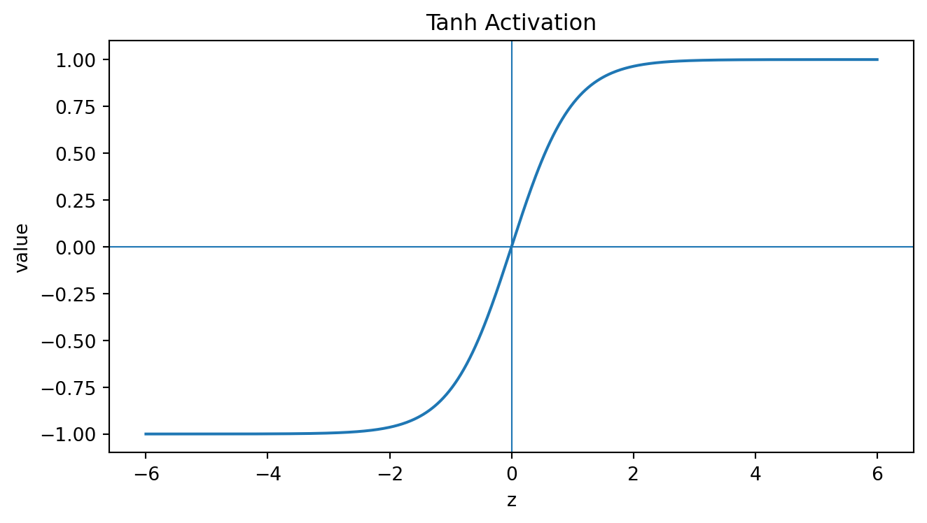
The hyperbolic tangent activation is

\[ \tanh(z) = \frac{e^{z}-e^{-z}}{e^z+e^{-z}} \]

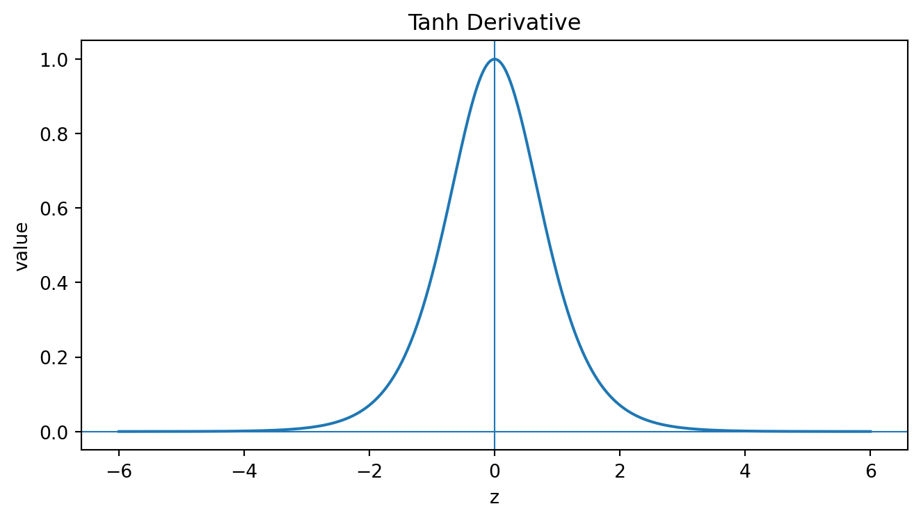
It maps real number to \((-1,1)\). Its derivative is

\[ \frac{d}{dz}\tanh(z) = 1-\tanh^2(z) \]

Compared with sigmoid, \(\tanh\) is zero-centered, which can help optimization in some settings. However, it also saturates for large positive or negative values of \(z\).

Show code
tanh = np.tanh(z)
tanh_deriv = 1 - tanh**2

for y, title in [
    (tanh, "Tanh Activation"),
    (tanh_deriv, "Tanh Derivative"),
]:
    plt.figure(figsize=(7, 4))
    plt.plot(z, y)
    plt.axhline(0, linewidth=0.8)
    plt.axvline(0, linewidth=0.8)
    plt.title(title)
    plt.xlabel("z")
    plt.ylabel("value")
    plt.tight_layout()
    plt.show()

2.3.3. Rectified Linear Unit

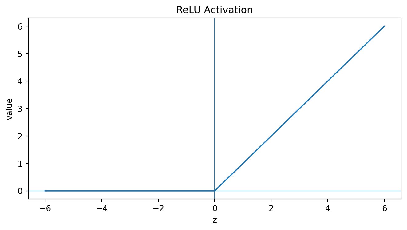
The Rectified Linear Unit, or ReLU, is

\[ ReLU(z) = \max (0, z) \]

Equivalently,

\[ ReLU(z) = \begin{cases}0, & z\leq 0\\ z,& z> 0\end{cases} \]

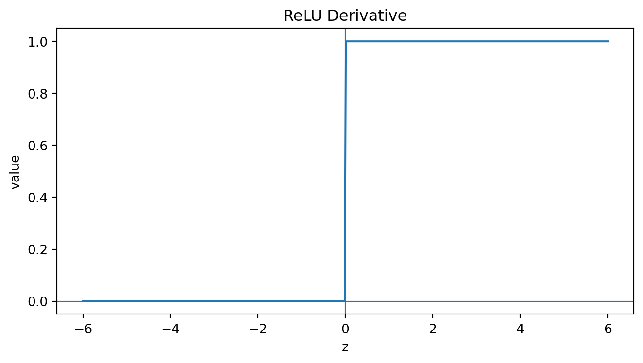
Its derivative is

\[ ReLU'(z) = \begin{cases}0, &z<0\\1,&z>0\end{cases} \]

At \(z=0\), the derivative is undefined, but in practice one chooses a subgradient, often 0 or 1.

ReLU became a standard activation in deep learning because it is computationally simple and helps reduce gradient for positive activations. However, ReLU units can “die” if they remain inactive, meaning their pre-activations stay negative and their gradients remain zero.

Show code
relu = np.maximum(0, z)
relu_deriv = (z > 0).astype(float)

for y, title in [
    (relu, "ReLU Activation"),
    (relu_deriv, "ReLU Derivative")
]:
    plt.figure(figsize=(7, 4))
    plt.plot(z, y)
    plt.axhline(0, linewidth=0.8)
    plt.axvline(0, linewidth=0.8)
    plt.title(title)
    plt.xlabel("z")
    plt.ylabel("value")
    plt.tight_layout()
    plt.show()

2.3.4 Softmax Function

For multiclass classification with \(K\) classes, the output layer often uses the softmax function. Given logits \(z=(z_1, z_2, \dots, z_K)\), the softmax output for class \(k\) is

\[ softmax(z)_k = \frac{e^{z_k}}{\sum_{j=1}^K e^{z_j}} \]

The softmax outputs satisfy \[ 0<softmax(z)_k<1\quad \text{and}\quad \sum_{k=1}^Ksoftmax(z)_k=1. \]

Thus, softmax transforms logits into a probability distribution over classes.

3. Multilayer Perceptions

3.1. Feedforward Neural Networks

A feedforward neural network, also called a multilayer perception, or MLP, is a composition of layer transformations.

Let \(a^{(0)}= x\) be the input vector. For layer \(l = 1, \dots, L,\) define

\[ z^{(l)}=W^{(l)}a^{(l-1)}+b^{(l)} \quad \text{and}\quad a^{(l)}=\sigma^{(l)}(z^{(l)}). \]

Here:

  • \(W^{(l)}\) is the weight matrix of layer \(l\),
  • \(b^{(l)}\) is the bias vector,
  • \(z^{(l)}\) is the pre-activation vector,
  • \(a^{(l)}\) is the activation vector.

The final output is

\[ \hat y = a^{(L)}. \]

Thus, the whole network is the composition

\[ f_\theta(x) = \sigma^{(L)}(W^{(L)}\sigma^{(L-1)}(W^{(L-1)}\cdots\sigma^{(1)}(W^{(1)}x+b^{(1)}))+b^{(L)}) \]

3.2. Dimensional Notation

Suppose layer \(l-1\) has \(d_{l-1}\) units and layer \(l\) has \(d_l\) units. Then

\[ \begin{aligned} a^{(l-1)}&\in \mathbb R^{d_{l-1}},\\ W^{(l)}&\in \mathbb R^{d_l \times d_{l-1}},\\ b^{(l)}&\in \mathbb R^{d_l},\\ z^{(l)}&\in \mathbb R^{d_l},\\ a^{(l)} &\in \mathbb R^{d_l} \end{aligned} \]

The number of parameters in layer \(l\) is

\[ d_ld_{l-1}+ d_l = d_l(d_{l-1}+1) \]

The total number of parameters in the network is

\[ P=\sum_{l=1}^L d_l(d_{l-1}+1) \]

ImportantExercise

Determine the number of trainable parameters of the following neural net:

  • Input layer: 4 units.
  • Hidden layer 1: 16 units.
  • Hidden layer 2: 8 units.
  • Hidden layer 3: 4 units.
  • Output layer: 2 units.
TipSolution

The number of trainable parameters between input layer and hidden layer 1 is \(16(4+1)=80.\)

The number of trainable parameters between hid.layer 1 and hid.layer 2 is \(8(16+1)=136.\)

The number of trainable parameters of hid.layer 2 and hid.layer 3 is \(4(8+1)=36.\)

The number of trainable parameters of hid.layer 3 and output layer is \(2(4+1)=10.\)

The total number of trainable parameters of the neural net is \(80+136+36+10=262.\)

3.3. Universal Approximation Theorem

NoteTheorem: Universal Approximation

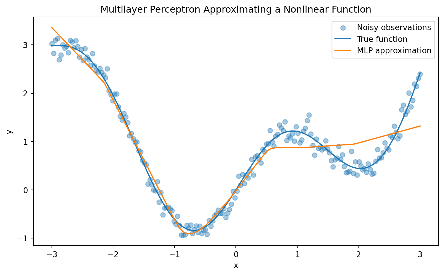
Let \(K\in \mathbb R^d\) be compact and let \(f: K\to \mathbb R\) be continuous. Under suitable conditions on the activation function, for every \(\epsilon > 0\), there exists a feedforward neural network \(g\) with at least one hidden layer such that:

\[ \sup_{x\in K} |f(x) - g(x)| <\epsilon \]

This theorem says that neural networks are capable of approximating continuous functions arbitrarily well on compact domains, provided the network is sufficiently large.

Show code
import numpy as np
import matplotlib.pyplot as plt
from sklearn.neural_network import MLPRegressor

rng = np.random.default_rng(42)

X = np.linspace(-3, 3, 200).reshape(-1, 1)
y_true = np.sin(2 * X).ravel() + 0.3 * X.ravel()**2
y = y_true + rng.normal(0, 0.15, size=X.shape[0])

model = MLPRegressor(
    hidden_layer_sizes=(50, 50),
    activation="relu",
    solver="adam",
    max_iter=3000,
    random_state=42
)

model.fit(X, y)

X_grid = np.linspace(-3, 3, 500).reshape(-1, 1)
y_pred = model.predict(X_grid)

plt.figure(figsize=(8, 5))
plt.scatter(X, y, alpha=0.4, label="Noisy observations")
plt.plot(X_grid, np.sin(2 * X_grid).ravel() + 0.3 * X_grid.ravel()**2, label="True function")
plt.plot(X_grid, y_pred, label="MLP approximation")
plt.title("Multilayer Perceptron Approximating a Nonlinear Function")
plt.xlabel("x")
plt.ylabel("y")
plt.legend()
plt.tight_layout()
plt.show()

4. Loss Functions

4.1. Regression Loss

For regression, the output is continuous \(y_i\in \mathbb R\). A common loss function is mean squared error:

\[ J(\theta) = \frac{1}{2n}\sum_{i=}^n(y_i-\hat y_i)^2, \]

where \(\hat y_i = f_\theta(x_i)\).

The factor \(\frac{1}{2}\) is often included because it simplifies derivatives:

\[ \frac{d}{d\hat y} \frac{1}{2}(y-\hat y)^2 =\hat y- y. \]

4.2. Binary Classification Loss

For binary classification \(y_i\in \{0,1\}\), the output layer often uses a sigmoid:

\[ \hat p_i=\sigma(z_i) = P(Y_i=1|x_i) \]

The binary cross-entropy loss is

\[ J(\theta) = -\frac{1}{n}\sum_{i=1}^n\left[y_i\log(\hat p_i)+(1-y_i)\log(1-\hat p_i)\right]. \]

TipMaximum Likelihood Interpretation

Assume \(Y_i \,|\, x_i\sim \text {Bernoulli} (\hat p_i)\), then

\[ P(Y_i = y_i\,|\, x_i) =\hat p_i^{y_i}(1-\hat p_i)^{1-y_i}. \]

The likelihood is

\[ L(\theta) = \prod_{i=1}^n \hat p_i^{y_i}(1-\hat p_i)^{1-y_i} \]

The log-likelihood is

\[ \ell(\theta) = \sum_{i=1}^n[y_i\log(\hat p_i)+(1-y_i)\log(1-\hat p_i)] \]

Maximizing \(\ell(\theta)\) is equivalent to minimizing \(-\ell(\theta)\), which is binary cross-entropy.

4.3. Multiclass Classification Loss

For multiclass classification \(y_i\in \{1, 2, \dots, K\}\), the network outputs logits \(z_i = (z_{i1}, \dots, z_{iK}).\) The softmax probability for class \(k\) is

\[ \hat p_{ik} = \frac{e^{z_{ik}}}{\sum_{j=1}^Ke^{z_{ij}}} \]

If the true label is represented as a one-hot vector \(y_i = (y_{i1},\dots, y_{iK})\), where \(y_{ik}=1\) if observation \(i\) belongs to class \(k\), then the multiclass corss-entropy loss is

\[ J(\theta) = -\frac{1}{n}\sum_{i=1}^n\sum_{k=1}^K y_{ik}\log (\hat p_{ik}) \]

If \(c_i\) is the true class index, this simplifies to

\[ J(\theta) = -\frac{1}{n} \sum_{i=1}^n \log (\hat p_{i, c_i}) \]

5. Backpropagation

Training a neural network means solving

\[ \theta = \arg\min_\theta J(\theta) \]

where \(\theta\) includes all weights and biases \(\theta = \{W^{(1)}, b^{(1)},\dots,W^{(L)}, b^{(L)}\}\). Because \(J(\theta)\) is usually nonconvex, closed-form solution are not available. Neural networks are trained with gradient-based optimization, requiring derivatives such as

\[ \frac{\partial J}{\partial W^{(l)}} \quad \text{and} \quad \frac{\partial J}{\partial b^{(l)}} \]

Backpropagation computes these derivatives efficiently using the chain rule.

5.1. Output-Layer Error

Consider one training example and define the loss \(\mathcal L\). For layer \(l\), define the error signal

\[ \delta^{(l)}=\frac{\partial \mathcal L}{\partial z^{(l)}}. \]

For the output layer \(L\),

\[ \delta ^{(L)} = \nabla_{a^{(L)}}\mathcal L \odot \sigma'^{(L)} (z^{(L)}), \]

where \(\odot\) denotes elementwise multiplication.

5.2. Hidden-Layer Backpropagation

For a hidden layer \(l\), the error signal is

\[ \delta^{(l)}=((W^{(l+1)})^\top\delta^{(l+1)})\odot \sigma'^{(l)}(z^{(l)}). \]

TipDerivation

We have

\[ z^{(l+1)}=W^{(l+1)}a^{(l)}+b^{(l+1)}, \qquad a^{(l)}=\sigma^{(l)}(z^{(l)}) \]

By the chain rule,

\[ \delta^{(l)}=\frac{\partial \mathcal L }{\partial z^{(l)}}=\frac{\partial \mathcal L}{\partial a^{(l)}}\frac{\partial a^{(l)}}{\partial z^{(l)}}=\frac{\partial \mathcal L}{\partial a^{(l)}}\odot \sigma'^{(l)}(z^{(l)}) \]

We also have:

\[ \frac{\partial \mathcal L}{\partial a^{(l)}}=\frac{\partial z^{(l+1)}}{\partial a^{(l)}}\frac{\partial \mathcal L}{\partial z^{(l+1)}}=(W^{(l+1)})^\top \frac{\partial \mathcal L}{\partial z^{(l+1)}}=(W^{(l+1)})^\top \delta^{(l+1)} \]

We obtain

\[ \delta^{(l)} = ((W^{(l+1)})^{\top} \delta^{(l+1)})\odot \sigma'^{(l)}(z^{(l)}) \]

5.3. Gradients with Respect to Weights and Biases

Since \(z^{(l)} = W^{(l)}a^{(l-1)}+b^{(l)}\), the gradients are

\[ \frac{\partial \mathcal L}{\partial W^{(l)}}=\delta^{(l)}(a^{(l-1)})^\top, \quad \text{and}\quad \frac{\partial \mathcal L}{\partial b^{(l)}}=\delta^{(l)} \]

For a mini-batch of \(m\) observations, gradients are averaged:

\[ \frac{\partial J}{\partial W^{(l)}}=\frac{1}{m}\sum_{i=1}^m \delta^{(l)}_i(a_i^{(l-1)})^\top \]

5.4. Gradient Descent Update

The standard gradient descent update is

\[ \begin{aligned} W^{(l)} &\leftarrow W^{(l)} - \alpha\frac{\partial J}{\partial W^{(l)}},\\ b^{(l)} &\leftarrow b^{(l)}-\alpha \frac{\partial J}{\partial b^{(l)}}. \end{aligned} \]

Here \(\alpha>0\) is the learning rate.

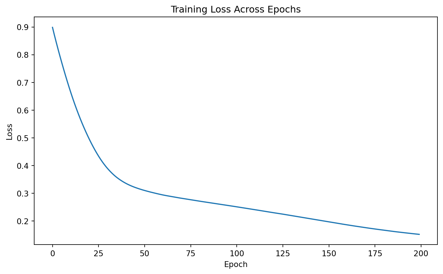
In stochastic gradient descent, the update uses one example or a mini-batch rather than the full dataset. Mini-batch training is standard in modern deep learning because it balances computational efficiency and gradient stability.

Show code
import numpy as np
import matplotlib.pyplot as plt
from sklearn.datasets import make_moons
from sklearn.neural_network import MLPClassifier
from sklearn.preprocessing import StandardScaler
from sklearn.pipeline import Pipeline

X, y = make_moons(n_samples=500, noise=0.25, random_state=42)

model = Pipeline([
    ("scaler", StandardScaler()),
    ("mlp", MLPClassifier(
        hidden_layer_sizes=(20, 20),
        activation="relu",
        solver="adam",
        max_iter=1,
        warm_start=True,
        random_state=42
    ))
])

losses = []

for epoch in range(200):
    model.fit(X, y)
    losses.append(model.named_steps["mlp"].loss_)

plt.figure(figsize=(8, 5))
plt.plot(losses)
plt.title("Training Loss Across Epochs")
plt.xlabel("Epoch")
plt.ylabel("Loss")
plt.tight_layout()
plt.show()

6. Optimization Challenges

6.1. Nonconvexity

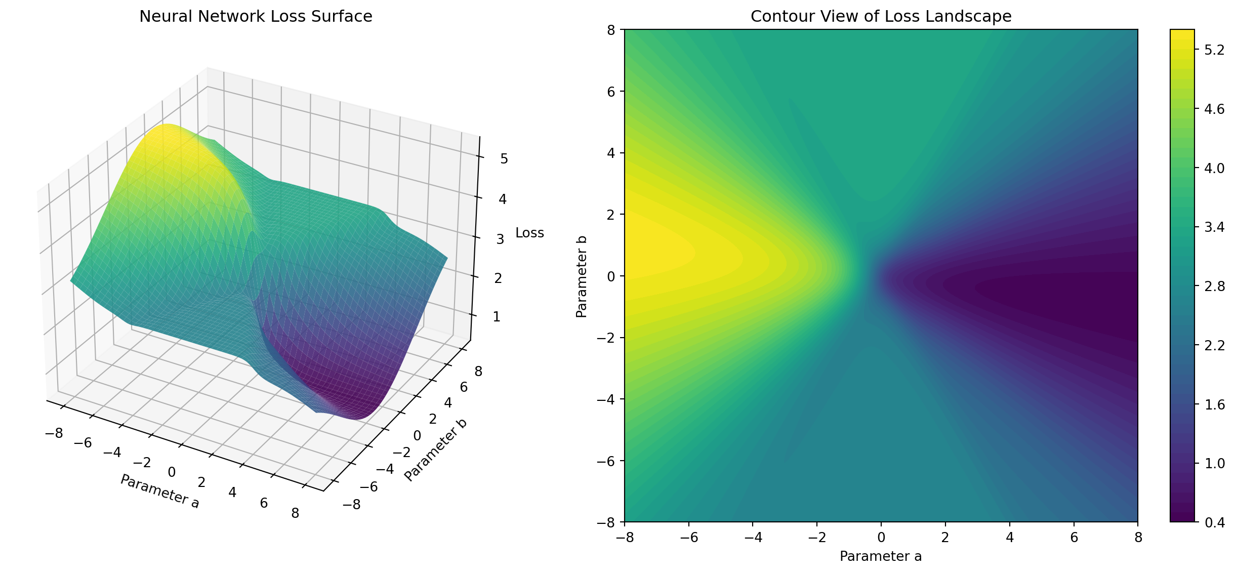
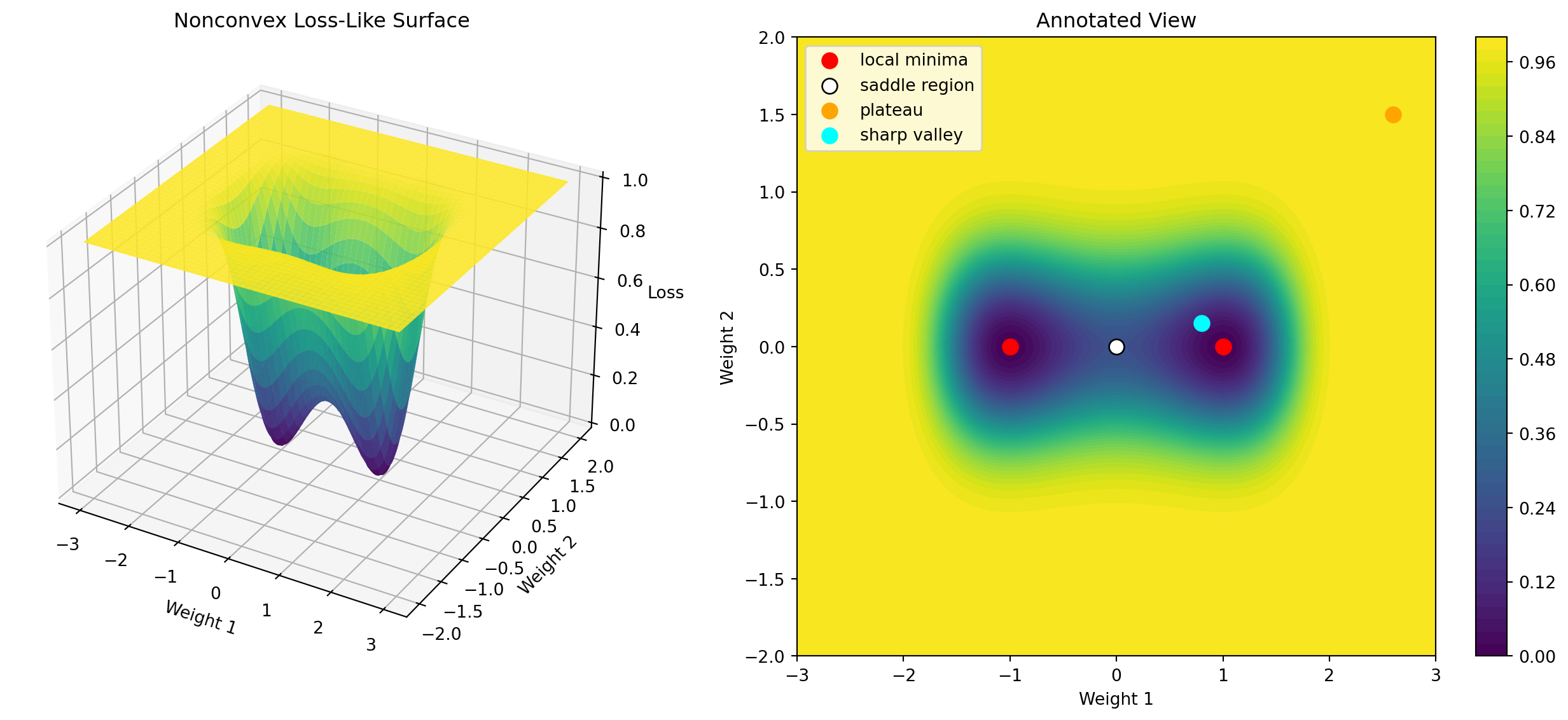
Unlike ordinary least squares regression, neural network training is generally nonconvex. The loss surface may contain local minima, saddle points, flat regions, sharp valleys, plateaus.

Show code
import numpy as np
import matplotlib.pyplot as plt

x = np.linspace(-2, 2, 100).reshape(-1, 1)
y = np.sin(3 * x)


def neural_net_prediction(x, a, b):
    """
    One-hidden-layer neural network:
    
    y_hat = c1*tanh(a*x + b)
          + c2*tanh(3*x - 1)
          + c3*tanh(-4*x + 0.5)
    
    Only a and b are changing.
    All other weights are fixed.
    """
    h1 = np.tanh(a * x + b)
    h2 = np.tanh(3 * x - 1)
    h3 = np.tanh(-4 * x + 0.5)
    
    y_hat = 1.2 * h1 - 0.7 * h2 + 0.5 * h3
    return y_hat

def loss(a, b):
    y_hat = neural_net_prediction(x, a, b)
    return np.mean((y_hat - y) ** 2)

a_values = np.linspace(-8, 8, 200)
b_values = np.linspace(-8, 8, 200)

A, B = np.meshgrid(a_values, b_values)
Z = np.zeros_like(A)

for i in range(A.shape[0]):
    for j in range(A.shape[1]):
        Z[i, j] = loss(A[i, j], B[i, j])

fig = plt.figure(figsize=(14, 6))

ax1 = fig.add_subplot(1, 2, 1, projection="3d")
ax1.plot_surface(A, B, Z, cmap="viridis", alpha=0.9)
ax1.set_title("Neural Network Loss Surface")
ax1.set_xlabel("Parameter a")
ax1.set_ylabel("Parameter b")
ax1.set_zlabel("Loss")

ax2 = fig.add_subplot(1, 2, 2)
contour = ax2.contourf(A, B, Z, levels=50, cmap="viridis")
plt.colorbar(contour, ax=ax2)
ax2.set_title("Contour View of Loss Landscape")
ax2.set_xlabel("Parameter a")
ax2.set_ylabel("Parameter b")

plt.tight_layout()
plt.show()

Show code
import numpy as np
import matplotlib.pyplot as plt

w1 = np.linspace(-3, 3, 300)
w2 = np.linspace(-2, 2, 300)
W1, W2 = np.meshgrid(w1, w2)

Z = np.tanh(((W1**2 - 1)**2 + 8 * W2**2) / 4)

fig = plt.figure(figsize=(14, 6))

ax1 = fig.add_subplot(1, 2, 1, projection="3d")
ax1.plot_surface(W1, W2, Z, cmap="viridis", alpha=0.9)
ax1.set_title("Nonconvex Loss-Like Surface")
ax1.set_xlabel("Weight 1")
ax1.set_ylabel("Weight 2")
ax1.set_zlabel("Loss")

ax2 = fig.add_subplot(1, 2, 2)
contour = ax2.contourf(W1, W2, Z, levels=60, cmap="viridis")
plt.colorbar(contour, ax=ax2)

ax2.scatter([-1, 1], [0, 0], s=80, color="red", label="local minima")
ax2.scatter([0], [0], s=80, color="white", edgecolor="black", label="saddle region")
ax2.scatter([2.6], [1.5], s=80, color="orange", label="plateau")
ax2.scatter([0.8], [0.15], s=80, color="cyan", label="sharp valley")

ax2.set_title("Annotated View")
ax2.set_xlabel("Weight 1")
ax2.set_ylabel("Weight 2")
ax2.legend()

plt.tight_layout()
plt.show()

The objective \(J(\theta)\) is nonconvex because the parameter appear inside nested nonlinear compositions. This does not mean neural network cannot be trained. In practice, stochastic gradient methods often find useful solution, especially in overparameterized networks. But it does mean that training depends a lot on initialization, learning rate, architecture, optimization algorithm, and regularization.

6.2. Vanishing and Exploding Gradients

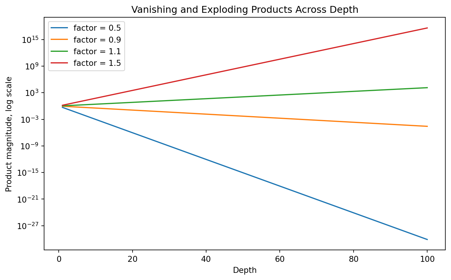
In deep networks, backpropagation repeatedly multiplies by weight matrices and activation derivatives. For a simplified scalar chain,

\[ \frac{\partial \mathcal L}{\partial z^{(1)}}=\frac{\partial \mathcal L}{\partial z^{(L)}}\prod_{l=2}^Lw^{(l)}\sigma'(z^{(l-1)}). \]

If the factor have magnitude less than 1, the product can shrink toward zero. This is the vanishing gradient problem. If the factors have magnitude greater than 1, the product can grow rapidly. This is the exploding gradient problem.

These problems are especially important in recurrent networks, where the same transformations is repeatedly applied overtime.

Show code
import numpy as np
import matplotlib.pyplot as plt

depth = np.arange(1, 101)

values = {
    "factor = 0.5": 0.5 ** depth,
    "factor = 0.9": 0.9 ** depth,
    "factor = 1.1": 1.1 ** depth,
    "factor = 1.5": 1.5 ** depth
}

plt.figure(figsize=(8, 5))
for label, vals in values.items():
    plt.plot(depth, vals, label=label)

plt.yscale("log")
plt.title("Vanishing and Exploding Products Across Depth")
plt.xlabel("Depth")
plt.ylabel("Product magnitude, log scale")
plt.legend()
plt.tight_layout()
plt.show()

7. Regularization and Generalization

A neural network may contain many more parameters than training observations. Such a model can memorize training data rather than generalize. Overfitting occurs wen training error decreases but validation error increases.

Mathematically, the empirical risk

\[ \hat R_n(\theta)=\frac{1}{n}\sum_{i=1}^n\mathcal L(y_i, f_\theta(x_i)) \]

may become small, while the expected risk

\[ R(\theta)=\mathbb E[\mathcal L(Y, f_\theta(X))] \]

remains large. Regularization methods attempt to reduce this gap.

7.1. Weight Decay

Weight decay, or \(L_2\) regularization, adds a penalty on parameter magnitude:

\[ J_\lambda = J(\theta)+\lambda\sum_{l=1}^L\|W^{(l)}\|_F^2 \]

Here \(\|W\|_F^2 = \sum_{i,j} W^2_{i,j}\). This discourages overly large weights and can improve generalization.

7.2. Dropout

Dropout randomly disable units during training. Let \(m^{(l)}\) be a random binary mask where each component is sampled as \(m_j^{(l)}\sim \text{Bernoulli}(q),\) which keep probability \(q=1-p\). The dropout activation is

\[ \tilde a^{(l)} = \frac{m^{(l)}\odot a^{(l)}}{q} \]

The scaling by \(1/q\) keeps the expected activation approximately unchanged:

\[ \mathbb E[\tilde a^{(l)}]=\mathbb E\left[\frac{m^{(l)}\odot a^{(l)}}{q}\right]=a^{(l)} \]

Dropout can be interpreted as training an implicit ensemble of subnetworks.

7.3. Early Stopping

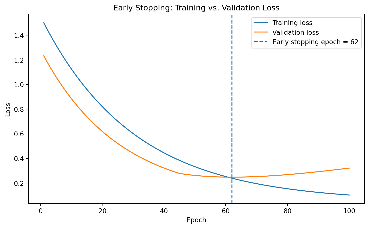
Early stopping monitors validation loss during training. If validation loss stops improving, training is halted.

Let \(J_{\text{train}}^{(t)}\) and \(J_\text{val}^{(t)}\) be the training and validation losses at epoch \(t\). Overfitting is suggested when \(J_{\text{train}}^{(t)}
\downarrow\) but \(J_{\text{val}}^{(t)}
\uparrow.\) Early stopping chooses parameters from an earlier epoch:

\[ \hat \theta = \theta^{(t^*)}, \quad \text{where } t^*=\arg\min_t J^{(t)}_\text{val}. \]

Show code
import numpy as np
import matplotlib.pyplot as plt

epochs = np.arange(1, 101)

train_loss = 1.5 * np.exp(-epochs / 30) + 0.05
val_loss = 1.2 * np.exp(-epochs / 25) + 0.004 * np.maximum(epochs - 45, 0) + 0.08

best_epoch = epochs[np.argmin(val_loss)]

plt.figure(figsize=(8, 5))
plt.plot(epochs, train_loss, label="Training loss")
plt.plot(epochs, val_loss, label="Validation loss")
plt.axvline(best_epoch, linestyle="--", label=f"Early stopping epoch = {best_epoch}")
plt.title("Early Stopping: Training vs. Validation Loss")
plt.xlabel("Epoch")
plt.ylabel("Loss")
plt.legend()
plt.tight_layout()
plt.show()

8. Specialized Neural Network Architectures

8.1. Convolutional Neural Networks

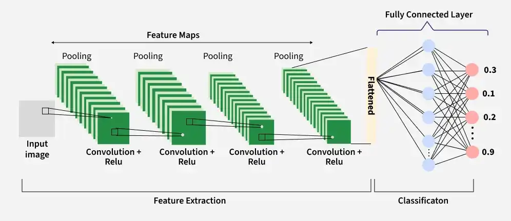
Convolutional Neural Networks, or CNNs, are designed for spatially structured data such as images. Their central idea is that local patterns should be detected using shared filters.

Convolutional Neural Network Architecture

For a one-dimensional signal \(x\) and filter \(w\), convolution can be written as

\[ z_t=\sum_{r=0}^{k-1} w_r x_{t+r} \]

For a two-dimensional image \(X\) and filter \(W\), convolution is

\[ Z_{i,j} = \sum_{w=0}^{h-1}\sum_{v=0}^{w-1} W_{u,v}X_{i+u, j+v} \]

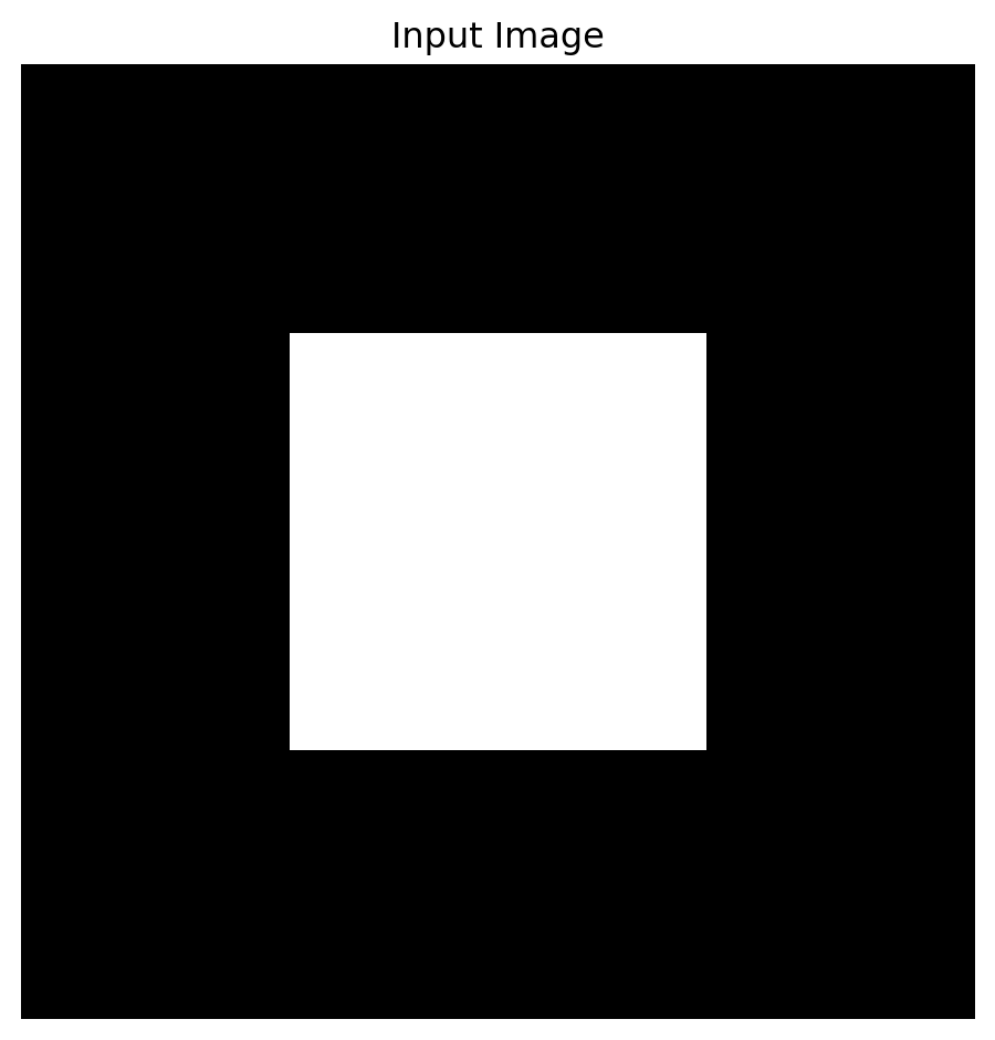
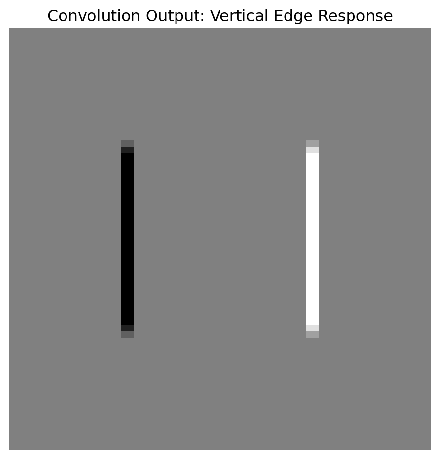
A convolutional layer learns filters that detect local features such as edges, corners, textures, or object parts.

CNNs typically use:

  1. Convolutional layers to extract local patterns.
  2. Activation functions to introduce nonlinearity.
  3. Pooling layers to reduce spatial resolution.
  4. Dense layers for final prediction.
NoteDefinition: Max Pooling

For a pooling window \(P_{i,j}\), max pooling computes

\[ M_{i,j} = \max_{(u,v)\in P_{i,j}} A_{u,v} \]

Pooling reduces spatial size and gives partial invariance to small translations.

Show code
import numpy as np
import matplotlib.pyplot as plt
from scipy.signal import convolve2d

# Create a simple image: white square on black background
image = np.zeros((64, 64))
image[18:46, 18:46] = 1

# Sobel-like vertical edge filter
kernel = np.array([
    [-1, 0, 1],
    [-2, 0, 2],
    [-1, 0, 1]
])

filtered = convolve2d(image, kernel, mode="same", boundary="fill")

plt.figure(figsize=(5, 5))
plt.imshow(image, cmap="gray")
plt.title("Input Image")
plt.axis("off")
plt.tight_layout()
plt.show()

plt.figure(figsize=(5, 5))
plt.imshow(filtered, cmap="gray")
plt.title("Convolution Output: Vertical Edge Response")
plt.axis("off")
plt.tight_layout()
plt.show()

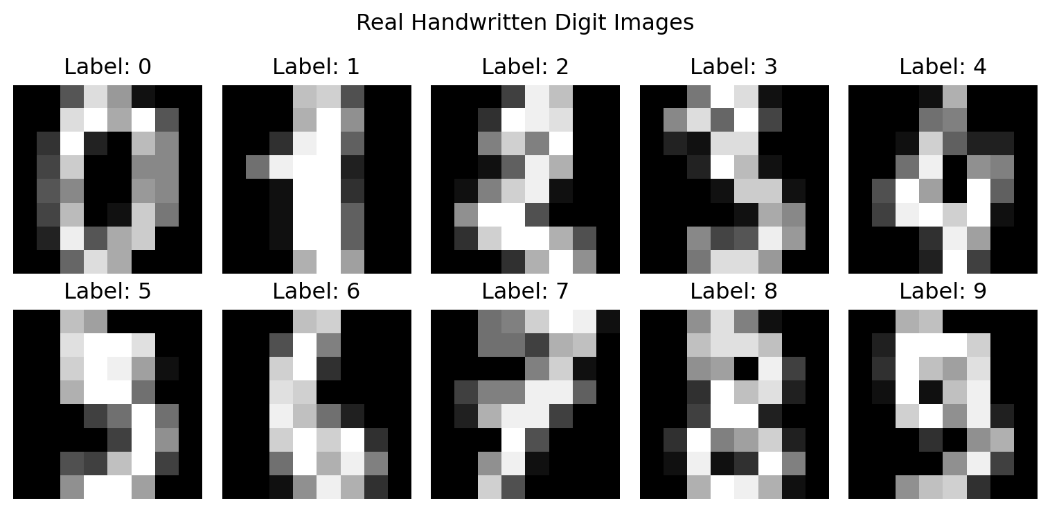
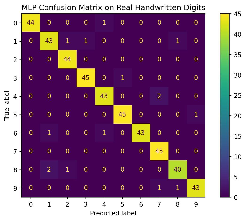
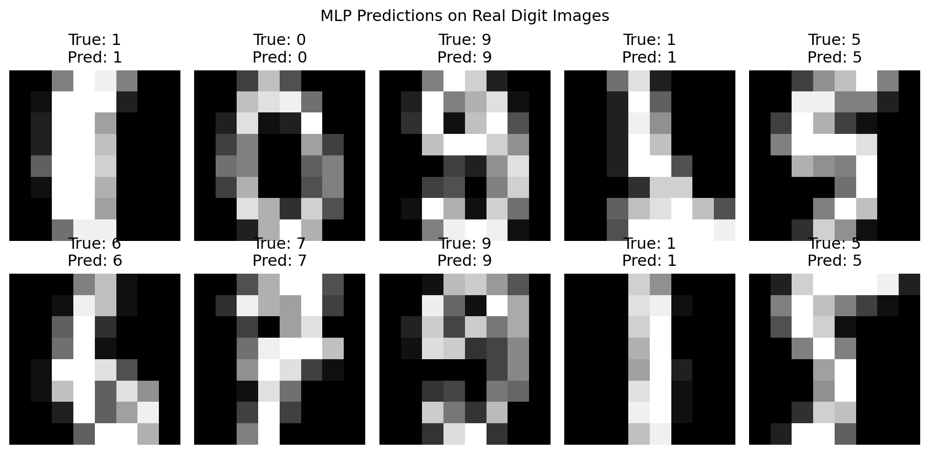
We then play again with the handwritten digit recognition from scikit-learn.

Show code
import numpy as np
import matplotlib.pyplot as plt
from sklearn.datasets import load_digits
from sklearn.neural_network import MLPClassifier
from sklearn.model_selection import train_test_split
from sklearn.preprocessing import StandardScaler
from sklearn.pipeline import Pipeline
from sklearn.metrics import ConfusionMatrixDisplay, accuracy_score

digits = load_digits()

X = digits.data
y = digits.target
images = digits.images

# Display real digit images
plt.figure(figsize=(8, 4))
for i in range(10):
    plt.subplot(2, 5, i + 1)
    plt.imshow(images[i], cmap="gray")
    plt.title(f"Label: {y[i]}")
    plt.axis("off")
plt.suptitle("Real Handwritten Digit Images")
plt.tight_layout()
plt.show()

X_train, X_test, y_train, y_test, images_train, images_test = train_test_split(
    X, y, images,
    test_size=0.25,
    random_state=42,
    stratify=y
)

model = Pipeline([
    ("scaler", StandardScaler()),
    ("mlp", MLPClassifier(
        hidden_layer_sizes=(64, 32),
        activation="relu",
        solver="adam",
        max_iter=1000,
        random_state=42
    ))
])

model.fit(X_train, y_train)
y_pred = model.predict(X_test)

print("Test accuracy:", accuracy_score(y_test, y_pred))

ConfusionMatrixDisplay.from_predictions(y_test, y_pred)
plt.title("MLP Confusion Matrix on Real Handwritten Digits")
plt.tight_layout()
plt.show()

plt.figure(figsize=(10, 5))
for i in range(10):
    plt.subplot(2, 5, i + 1)
    plt.imshow(images_test[i], cmap="gray")
    plt.title(f"True: {y_test[i]}\nPred: {y_pred[i]}")
    plt.axis("off")
plt.suptitle("MLP Predictions on Real Digit Images")
plt.tight_layout()
plt.show()

Test accuracy: 0.9666666666666667

8.2. Recurrent Neural Networks

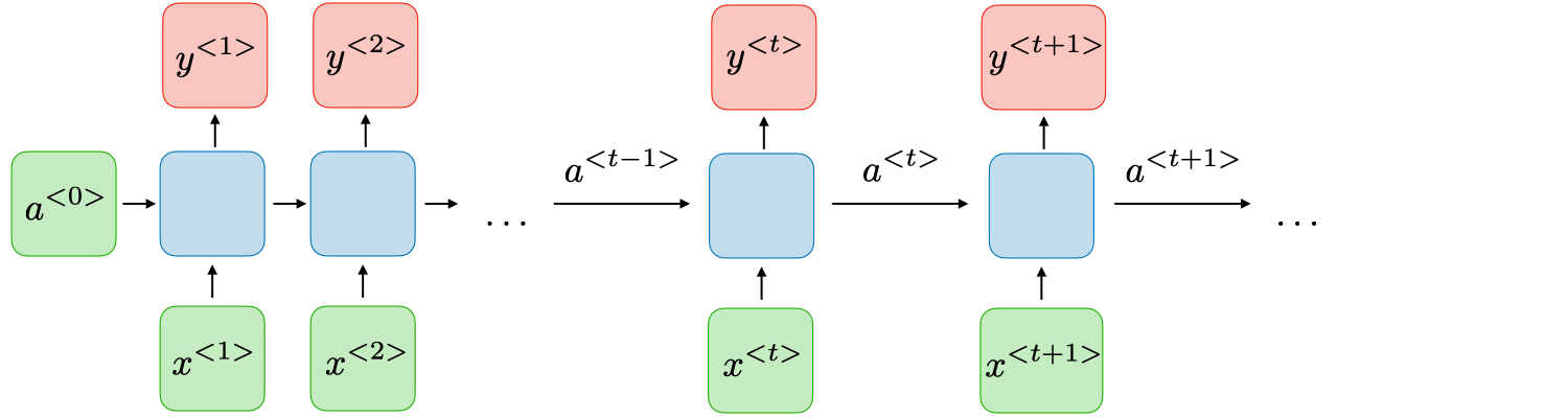
Recurrent Neural Networks, or RNNs, are designed for sequential data. They maintain a hidden state that evolves over time.

Recurrent Neural Network Architecture

Given an input sequence \(x_1, x_2, \cdots, x_T,\) an RNN computes

\[ h_t = \phi(W_x x_t + W_h h_{t-1}+b_h),\qquad \hat y_t=g(W_y h_t + b_y). \]

The hidden state \(h_t\) acts as a memory of previous inputs.

RNNs are useful for:

  • language modeling,
  • time series prediction,
  • speech recognition,
  • sequence labeling,
  • translation.

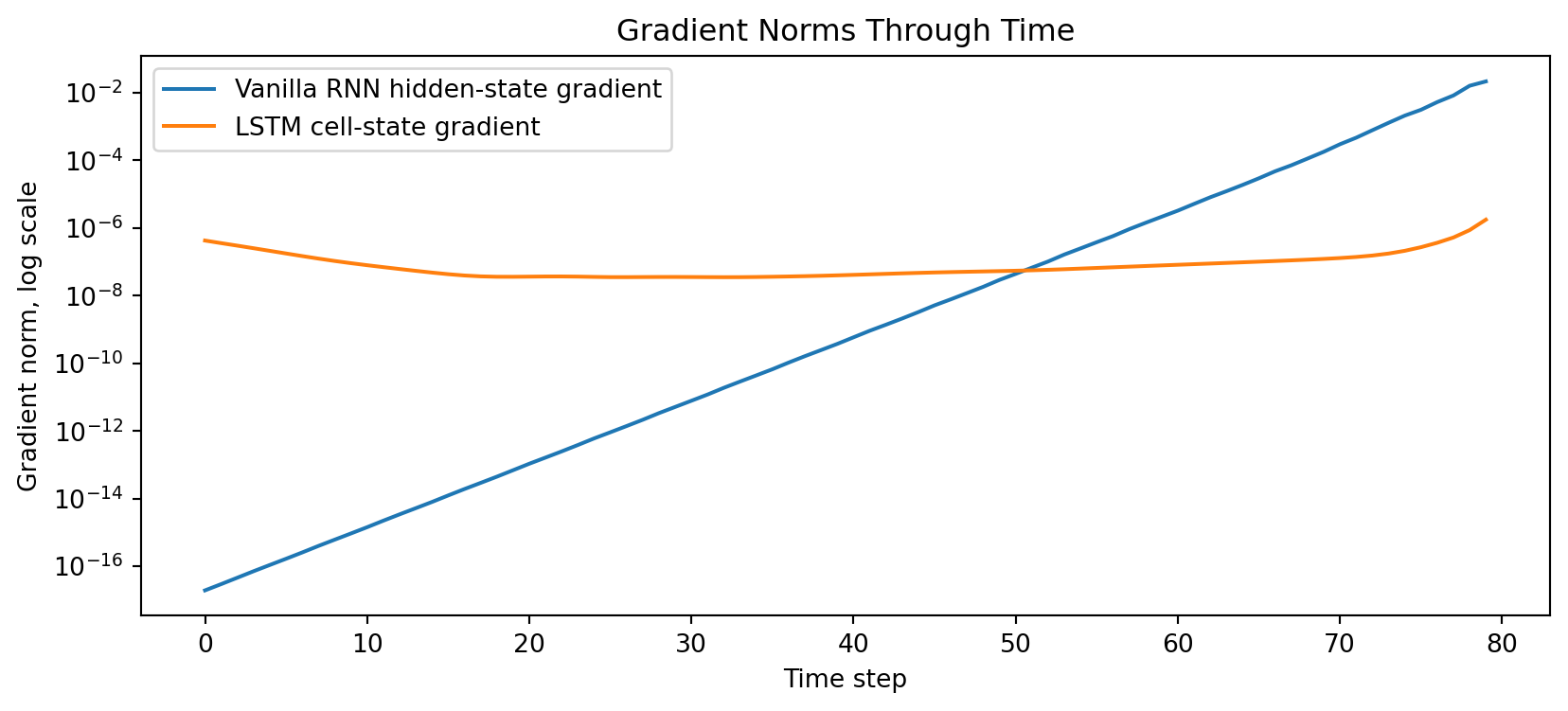
However, basic RNNs suffer from vanishing and exploding gradients because the same recurrent transformation is applied repeatedly over time.

8.3. Long Short-Term Memory Networks

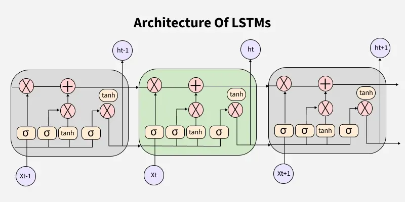
Long Short-Term Memory networks, or LSTMs, were introduced to address long-range dependency problems in recurrent networks. An LSTM maintains a cell state \(c_t\) controlled by gates.

Long Short-Term Memory Network Architecture

A standard LSTM uses:

  • Forget gate: \(f_t =\sigma(W_fx_t+ U_fh_{t-1}+b_f)\).
  • Input gate: \(i_i = \sigma(W_i x_t + U_i h_{t-1}+ b_i)\).
  • Output gate: \(o_t = \sigma (W_ox_t + U_oh_{t-1}+ b_o)\)
  • Candidate cell state: \(\tilde c_t = \tanh (W_c x_t + U_c h_{t-1}+ b_c)\)
  • Cell update: \(c_t= f_t\odot c_{t-1}+ i_t \odot \tilde c_t\)
  • Hidden state update: \(h_t=o_t\odot \tanh (c_t)\)

The cell state creates a pathway through time that helps preserve gradients over longer intervals.

Show code
import torch
import torch.nn as nn
import torch.optim as optim
import matplotlib.pyplot as plt

torch.manual_seed(42)
torch.set_num_threads(2)

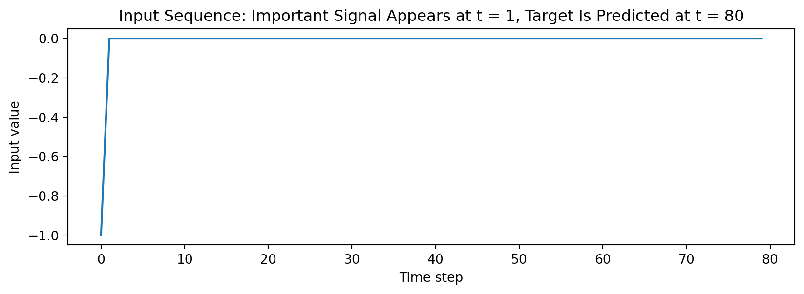
def generate_memory_batch(batch_size=128, seq_len=80):
    """
    Input:
        x_1 contains the important signal.
        x_2, ..., x_T are all zeros.

    Target:
        predict the original signal at the final time step.

    This tests whether the model can remember information from far in the past.
    """
    x = torch.zeros(batch_size, seq_len, 1)

    bit = torch.randint(0, 2, (batch_size, 1)).float()

    # Use -1 and +1 as the input signal
    x[:, 0, 0] = bit[:, 0] * 2 - 1

    # Classification target: 0 or 1
    y = bit

    return x, y


seq_len = 80

x_example, y_example = generate_memory_batch(batch_size=1, seq_len=seq_len)

plt.figure(figsize=(10, 3))
plt.plot(x_example[0, :, 0])
plt.title(f"Input Sequence: Important Signal Appears at t = 1, Target Is Predicted at t = {seq_len}")
plt.xlabel("Time step")
plt.ylabel("Input value")
plt.show()

print("Target:", int(y_example.item()))

Target: 0
Show code
class VanillaRNNClassifier(nn.Module):
    def __init__(self, hidden_size=32):
        super().__init__()

        self.rnn = nn.RNN(
            input_size=1,
            hidden_size=hidden_size,
            batch_first=True,
            nonlinearity="tanh"
        )

        self.output_layer = nn.Linear(hidden_size, 1)

    def forward(self, x):
        hidden_sequence, _ = self.rnn(x)

        # Use only the final hidden state
        final_hidden = hidden_sequence[:, -1, :]

        logit = self.output_layer(final_hidden)

        return logit
        
class LSTMClassifier(nn.Module):
    def __init__(self, hidden_size=32):
        super().__init__()

        self.lstm = nn.LSTM(
            input_size=1,
            hidden_size=hidden_size,
            batch_first=True
        )

        self.output_layer = nn.Linear(hidden_size, 1)

        # Helpful initialization:
        # Make the forget gate initially prefer remembering.
        with torch.no_grad():
            for name in ["bias_ih_l0", "bias_hh_l0"]:
                bias = getattr(self.lstm, name)

                # PyTorch LSTM gate order:
                # input gate, forget gate, cell gate, output gate
                hidden_size = self.lstm.hidden_size
                bias[hidden_size:2 * hidden_size].fill_(1.5)

    def forward(self, x):
        hidden_sequence, _ = self.lstm(x)

        # Use only the final hidden state
        final_hidden = hidden_sequence[:, -1, :]

        logit = self.output_layer(final_hidden)

        return logit

def train_model(model, epochs=300, lr=0.003, seq_len=80):
    loss_fn = nn.BCEWithLogitsLoss()
    optimizer = optim.Adam(model.parameters(), lr=lr)

    loss_history = []
    acc_history = []

    for epoch in range(epochs):
        x_batch, y_batch = generate_memory_batch(
            batch_size=128,
            seq_len=seq_len
        )

        logits = model(x_batch)
        loss = loss_fn(logits, y_batch)

        optimizer.zero_grad()
        loss.backward()

        # Prevent exploding gradients
        torch.nn.utils.clip_grad_norm_(model.parameters(), max_norm=1.0)

        optimizer.step()

        if epoch % 10 == 0:
            with torch.no_grad():
                x_test, y_test = generate_memory_batch(
                    batch_size=512,
                    seq_len=seq_len
                )

                test_logits = model(x_test)
                test_probs = torch.sigmoid(test_logits)
                test_preds = (test_probs > 0.5).float()

                acc = (test_preds == y_test).float().mean().item()

            loss_history.append(loss.item())
            acc_history.append(acc)

    return loss_history, acc_history
Show code
rnn_model = VanillaRNNClassifier(hidden_size=32)
lstm_model = LSTMClassifier(hidden_size=32)

rnn_losses, rnn_accs = train_model(
    rnn_model,
    epochs=300,
    lr=0.003,
    seq_len=seq_len
)

lstm_losses, lstm_accs = train_model(
    lstm_model,
    epochs=300,
    lr=0.003,
    seq_len=seq_len
)

print("Final RNN accuracy:", rnn_accs[-1])
print("Final LSTM accuracy:", lstm_accs[-1])
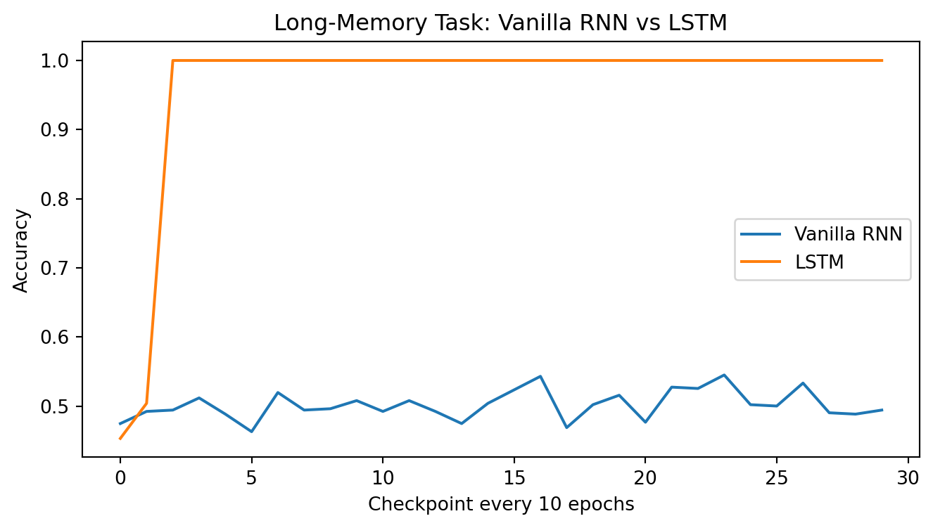
Final RNN accuracy: 0.494140625
Final LSTM accuracy: 1.0
Show code
plt.figure(figsize=(8, 4))
plt.plot(rnn_accs, label="Vanilla RNN")
plt.plot(lstm_accs, label="LSTM")
plt.title("Long-Memory Task: Vanilla RNN vs LSTM")
plt.xlabel("Checkpoint every 10 epochs")
plt.ylabel("Accuracy")
plt.legend()
plt.show()

Show code
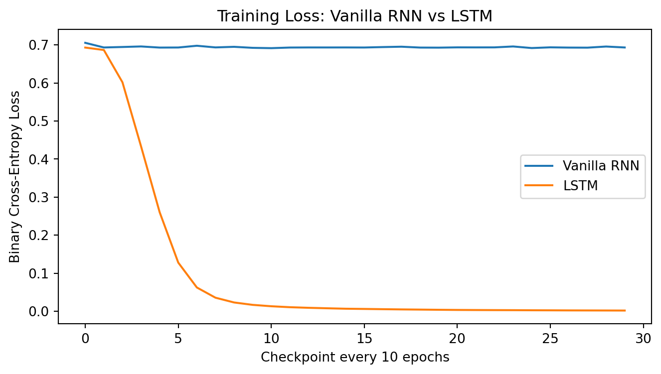
plt.figure(figsize=(8, 4))
plt.plot(rnn_losses, label="Vanilla RNN")
plt.plot(lstm_losses, label="LSTM")
plt.title("Training Loss: Vanilla RNN vs LSTM")
plt.xlabel("Checkpoint every 10 epochs")
plt.ylabel("Binary Cross-Entropy Loss")
plt.legend()
plt.show()

Show code
x_test, y_test = generate_memory_batch(batch_size=10, seq_len=seq_len)

with torch.no_grad():
    rnn_probs = torch.sigmoid(rnn_model(x_test))
    lstm_probs = torch.sigmoid(lstm_model(x_test))

print("True targets:")
print(y_test.squeeze().int().tolist())

print("\nRNN predicted probabilities:")
print(rnn_probs.squeeze().tolist())

print("\nLSTM predicted probabilities:")
print(lstm_probs.squeeze().tolist())
True targets:
[0, 0, 1, 0, 0, 0, 0, 1, 0, 1]

RNN predicted probabilities:
[0.5103229880332947, 0.5103229880332947, 0.5103229880332947, 0.5103229880332947, 0.5103229880332947, 0.5103229880332947, 0.5103229880332947, 0.5103229880332947, 0.5103229880332947, 0.5103229880332947]

LSTM predicted probabilities:
[0.001612615305930376, 0.001612615305930376, 0.9979119896888733, 0.001612615305930376, 0.001612615305930376, 0.001612615305930376, 0.001612615305930376, 0.9979119896888733, 0.001612615305930376, 0.9979119896888733]
Show code
def rnn_gradient_norms(model, seq_len=80):
    hidden_size = model.rnn.hidden_size

    cell = nn.RNNCell(
        input_size=1,
        hidden_size=hidden_size,
        nonlinearity="tanh"
    )

    # Copy trained RNN weights into an RNNCell so we can inspect each hidden state
    cell.weight_ih.data.copy_(model.rnn.weight_ih_l0.data)
    cell.weight_hh.data.copy_(model.rnn.weight_hh_l0.data)
    cell.bias_ih.data.copy_(model.rnn.bias_ih_l0.data)
    cell.bias_hh.data.copy_(model.rnn.bias_hh_l0.data)

    x, y = generate_memory_batch(batch_size=128, seq_len=seq_len)

    h = torch.zeros(x.shape[0], hidden_size)

    hidden_states = []

    for t in range(seq_len):
        h = cell(x[:, t, :], h)
        h.retain_grad()
        hidden_states.append(h)

    logit = model.output_layer(h)

    loss_fn = nn.BCEWithLogitsLoss()
    loss = loss_fn(logit, y)

    model.zero_grad()
    cell.zero_grad()
    loss.backward()

    grad_norms = []

    for h_t in hidden_states:
        grad_norms.append(h_t.grad.norm().item())

    return grad_norms


def lstm_gradient_norms(model, seq_len=80):
    hidden_size = model.lstm.hidden_size

    cell = nn.LSTMCell(
        input_size=1,
        hidden_size=hidden_size
    )

    # Copy trained LSTM weights into an LSTMCell
    cell.weight_ih.data.copy_(model.lstm.weight_ih_l0.data)
    cell.weight_hh.data.copy_(model.lstm.weight_hh_l0.data)
    cell.bias_ih.data.copy_(model.lstm.bias_ih_l0.data)
    cell.bias_hh.data.copy_(model.lstm.bias_hh_l0.data)

    x, y = generate_memory_batch(batch_size=128, seq_len=seq_len)

    h = torch.zeros(x.shape[0], hidden_size)
    c = torch.zeros(x.shape[0], hidden_size)

    cell_states = []

    for t in range(seq_len):
        h, c = cell(x[:, t, :], (h, c))
        c.retain_grad()
        cell_states.append(c)

    logit = model.output_layer(h)

    loss_fn = nn.BCEWithLogitsLoss()
    loss = loss_fn(logit, y)

    model.zero_grad()
    cell.zero_grad()
    loss.backward()

    grad_norms = []

    for c_t in cell_states:
        grad_norms.append(c_t.grad.norm().item())

    return grad_norms
    
rnn_grads = rnn_gradient_norms(rnn_model, seq_len=seq_len)
lstm_grads = lstm_gradient_norms(lstm_model, seq_len=seq_len)

plt.figure(figsize=(10, 4))
plt.plot(rnn_grads, label="Vanilla RNN hidden-state gradient")
plt.plot(lstm_grads, label="LSTM cell-state gradient")
plt.yscale("log")
plt.title("Gradient Norms Through Time")
plt.xlabel("Time step")
plt.ylabel("Gradient norm, log scale")
plt.legend()
plt.show()

8.4. Transformers and Attention

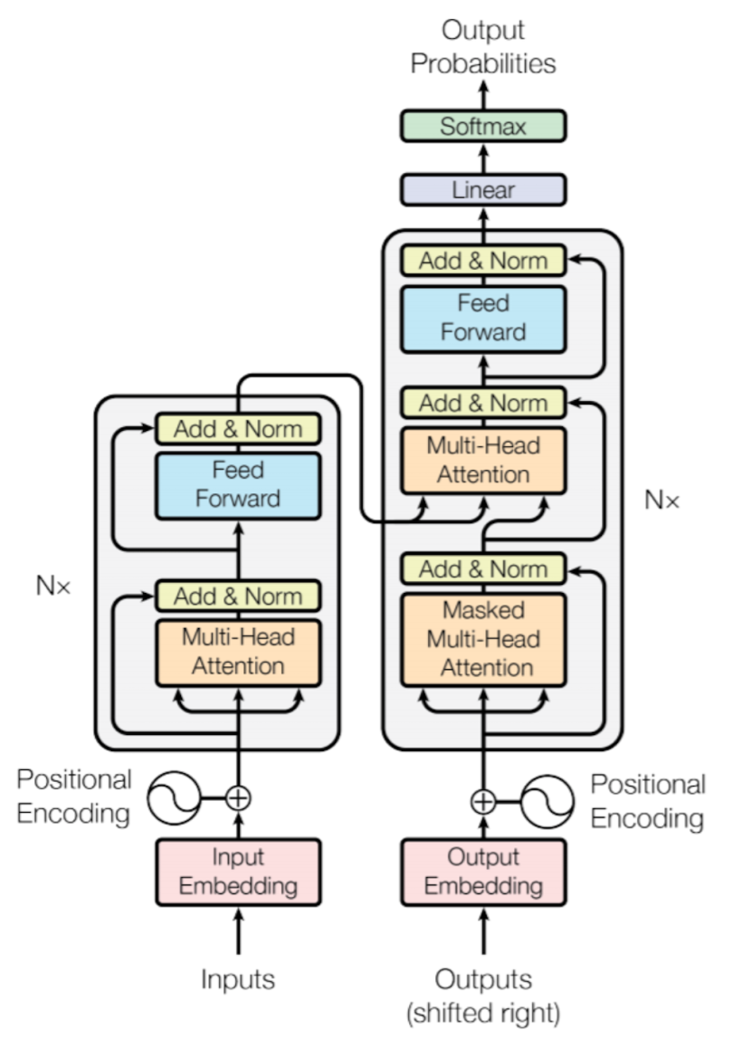
Transformers replace recurrence with attention mechanisms. Their central operation is scaled dot-product attention.

Transformers and Attention
NoteDefinition: Attention

Given matrices of queries \(Q\), keys \(K\), and values \(V\), attention is

\[ \text{Attention}(Q, K, V) =\text{softmax}\left(\frac{QK^\top}{\sqrt {d_k}}\right)V. \]

where:

  • \(Q\) represents what each token is looking for,
  • \(K\) represents what each token offers for matching,
  • \(V\) represents the information to be aggregated,
  • \(d_k\) is the key dimension.

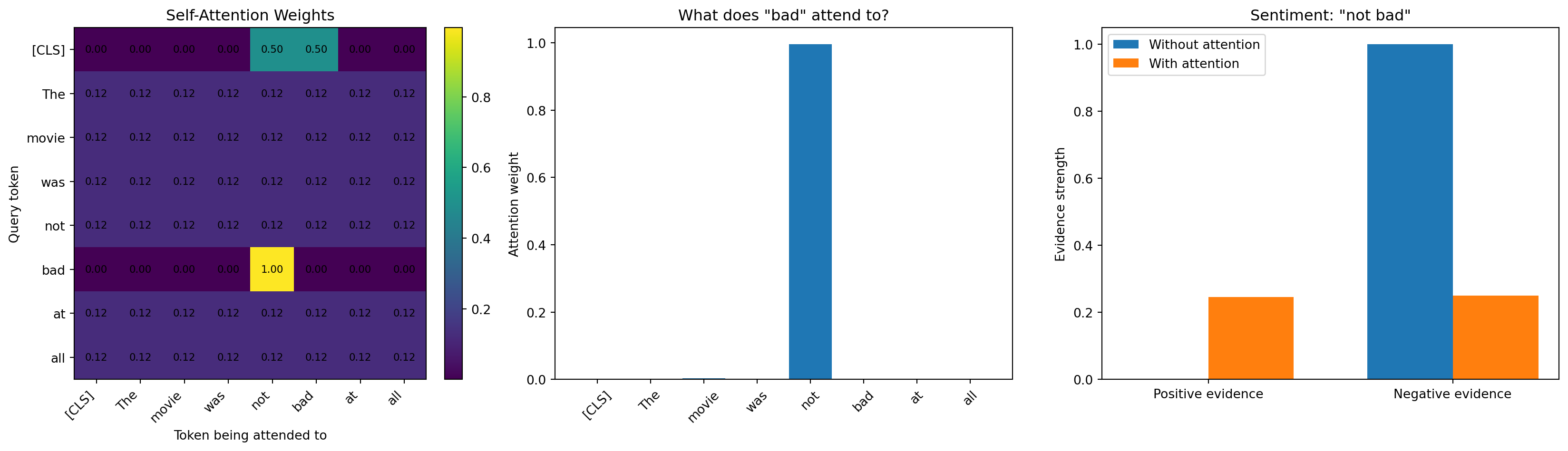
The matrix \(\text{softmax}\left(\frac{QK^\top}{\sqrt{d_k}}\right)\) contains attention weights showing how much each token attends to each other token. Transformers are powerful because they allow every token in a sequence to interact with every other token directly, rather than passing information step by step through recurrent states.

Show code
import numpy as np
import matplotlib.pyplot as plt

def softmax(x, axis=-1):
    x = x - np.max(x, axis=axis, keepdims=True)
    exp_x = np.exp(x)
    return exp_x / np.sum(exp_x, axis=axis, keepdims=True)

tokens = ["[CLS]", "The", "movie", "was", "not", "bad", "at", "all"]
n_tokens = len(tokens)

# We create small query/key vectors by hand.
# This is for visualization, not real training.
d_k = 4

Q = np.zeros((n_tokens, d_k))
K = np.zeros((n_tokens, d_k))

# Index helpers
CLS = tokens.index("[CLS]")
NOT = tokens.index("not")
BAD = tokens.index("bad")
MOVIE = tokens.index("movie")

# Dimension meaning:
# dim 0: looking for negation
# dim 1: looking for sentiment words
# dim 2: looking for subject/context
# dim 3: filler/general matching

# "bad" looks strongly for negation
Q[BAD, 0] = 4.0
K[NOT, 0] = 4.0

# [CLS] looks for sentiment and negation because it represents the whole sentence
Q[CLS, 0] = 3.0
Q[CLS, 1] = 3.0
K[NOT, 0] = 4.0
K[BAD, 1] = 4.0

# "bad" also connects slightly to the subject "movie"
Q[BAD, 2] = 2.0
K[MOVIE, 2] = 2.0

# Add weak self-matching so each token still attends a little to itself
for i in range(n_tokens):
    Q[i, 3] = 0.5
    K[i, 3] = 0.5


scores = Q @ K.T / np.sqrt(d_k)
attention_weights = softmax(scores, axis=1)

# Value dimensions:
# [positive_feature, negative_feature, negation_feature]
V = np.zeros((n_tokens, 3))

V[NOT] = [0.0, 0.0, 1.0]   # "not" contributes negation
V[BAD] = [0.0, 1.0, 0.0]   # "bad" contributes negative meaning

# Context vectors after attention
context = attention_weights @ V

# Naive model sees "bad" and thinks negative
naive_positive = 0.0
naive_negative = 1.0

# Attention-aware model combines "not" and "bad"
cls_context = context[CLS]

positive_feature = cls_context[0]
negative_feature = cls_context[1]
negation_feature = cls_context[2]

# Simple toy rule:
# negative + negation becomes positive evidence
attention_positive = positive_feature + negative_feature * negation_feature
attention_negative = negative_feature * (1 - negation_feature)

fig, axes = plt.subplots(1, 3, figsize=(18, 5))

im = axes[0].imshow(attention_weights)
axes[0].set_title("Self-Attention Weights")
axes[0].set_xticks(range(n_tokens))
axes[0].set_yticks(range(n_tokens))
axes[0].set_xticklabels(tokens, rotation=45, ha="right")
axes[0].set_yticklabels(tokens)
axes[0].set_xlabel("Token being attended to")
axes[0].set_ylabel("Query token")

for i in range(n_tokens):
    for j in range(n_tokens):
        axes[0].text(j, i, f"{attention_weights[i, j]:.2f}",
                     ha="center", va="center", fontsize=8)

fig.colorbar(im, ax=axes[0], fraction=0.046, pad=0.04)

# Attention distribution from "bad"
axes[1].bar(tokens, attention_weights[BAD])
axes[1].set_title('What does "bad" attend to?')
axes[1].set_ylabel("Attention weight")
axes[1].tick_params(axis="x", rotation=45)

# Naive vs attention-aware sentiment evidence
labels = ["Positive evidence", "Negative evidence"]
naive_scores = [naive_positive, naive_negative]
attention_scores = [attention_positive, attention_negative]

x = np.arange(len(labels))
width = 0.35

axes[2].bar(x - width / 2, naive_scores, width, label="Without attention")
axes[2].bar(x + width / 2, attention_scores, width, label="With attention")

axes[2].set_title('Sentiment: "not bad"')
axes[2].set_xticks(x)
axes[2].set_xticklabels(labels)
axes[2].set_ylabel("Evidence strength")
axes[2].legend()

plt.tight_layout()
plt.show()

8.5. Autoencoders

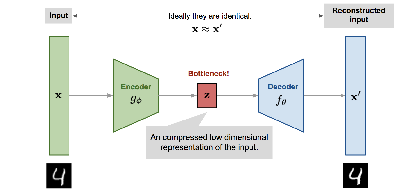
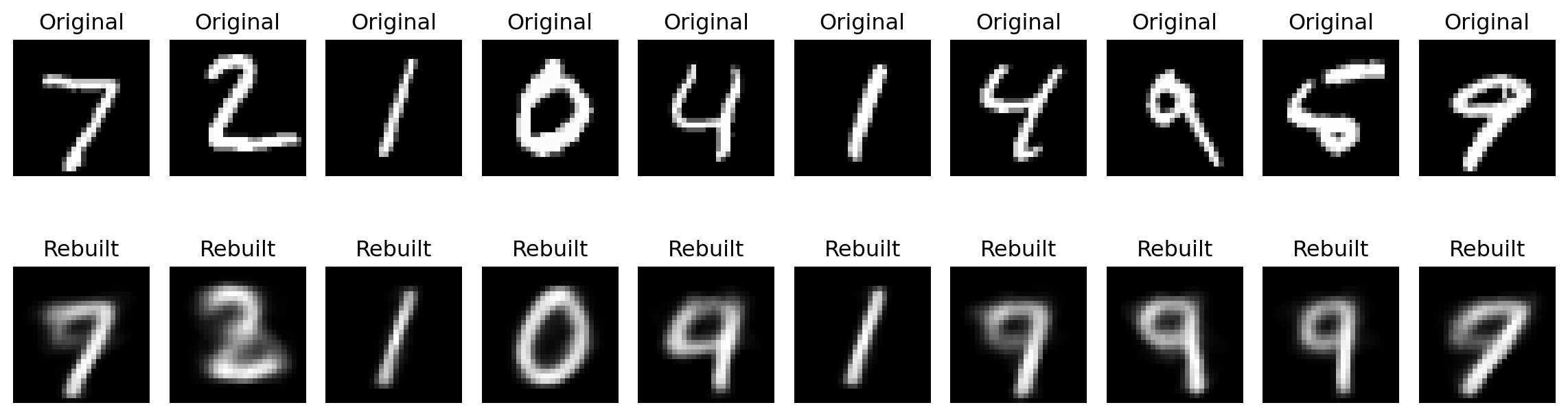
An autoencoders is an unsupervised neural network trained to reconstruct its input. It consists of an encoder and a decoder.

Autoencoders

The encoder maps input to latent representation \(h = g_\phi(x)\). The decoder maps latent representation back to reconstruction \(\hat x = r_\psi (h)\).

The training objective is

\[ \min_{\phi, \psi}\frac{1}{n}\sum_{i=1}^n\|x_i-r_\psi(g_\phi(x_i))\|^2. \]

If the latent space has lower dimension than the input, the network is forced to compress the data. This makes autoencoders useful for:

  • dimensionality reduction,
  • representation learning,
  • denoising,
  • anomaly detection.
Show code
# Simple Autoencoder on MNIST
# pip install torch torchvision matplotlib

import torch
import torch.nn as nn
import torch.optim as optim
import matplotlib.pyplot as plt

from torchvision import datasets, transforms
from torch.utils.data import DataLoader

device = torch.device("cuda" if torch.cuda.is_available() else "cpu")

input_dim = 28 * 28
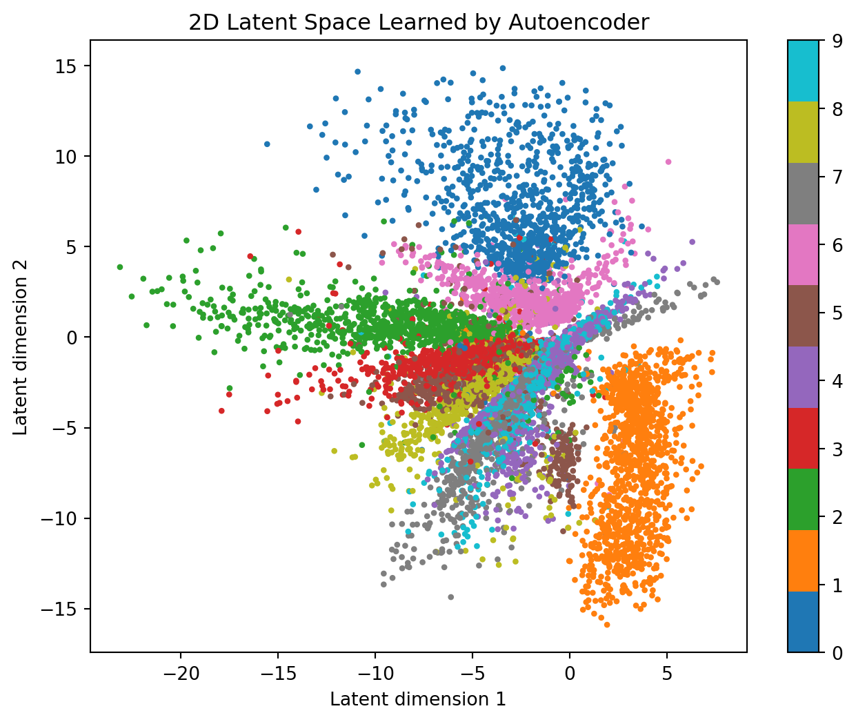
latent_dim = 2          # very small latent space for visualization
batch_size = 128
epochs = 10
lr = 0.001


transform = transforms.ToTensor()

train_dataset = datasets.MNIST(
    root="./data",
    train=True,
    transform=transform,
    download=True
)

test_dataset = datasets.MNIST(
    root="./data",
    train=False,
    transform=transform,
    download=True
)

train_loader = DataLoader(
    train_dataset,
    batch_size=batch_size,
    shuffle=True
)

test_loader = DataLoader(
    test_dataset,
    batch_size=batch_size,
    shuffle=False
)

class Autoencoder(nn.Module):
    def __init__(self, input_dim, latent_dim):
        super().__init__()

        # Encoder: x -> h
        self.encoder = nn.Sequential(
            nn.Linear(input_dim, 256),
            nn.ReLU(),

            nn.Linear(256, 64),
            nn.ReLU(),

            nn.Linear(64, latent_dim)
        )

        # Decoder: h -> x_hat
        self.decoder = nn.Sequential(
            nn.Linear(latent_dim, 64),
            nn.ReLU(),

            nn.Linear(64, 256),
            nn.ReLU(),

            nn.Linear(256, input_dim),
            nn.Sigmoid()   # output between 0 and 1
        )

    def forward(self, x):
        h = self.encoder(x)
        x_hat = self.decoder(h)
        return x_hat, h


model = Autoencoder(input_dim, latent_dim).to(device)

criterion = nn.MSELoss()
optimizer = optim.Adam(model.parameters(), lr=lr)

for epoch in range(epochs):
    model.train()
    total_loss = 0

    for images, _ in train_loader:
        images = images.view(-1, input_dim).to(device)

        reconstructed, latent = model(images)

        loss = criterion(reconstructed, images)

        optimizer.zero_grad()
        loss.backward()
        optimizer.step()

        total_loss += loss.item()

    avg_loss = total_loss / len(train_loader)

    print(f"Epoch [{epoch + 1}/{epochs}], Reconstruction Loss: {avg_loss:.4f}")
Epoch [1/10], Reconstruction Loss: 0.0610
Epoch [2/10], Reconstruction Loss: 0.0483
Epoch [3/10], Reconstruction Loss: 0.0447
Epoch [4/10], Reconstruction Loss: 0.0430
Epoch [5/10], Reconstruction Loss: 0.0419
Epoch [6/10], Reconstruction Loss: 0.0411
Epoch [7/10], Reconstruction Loss: 0.0404
Epoch [8/10], Reconstruction Loss: 0.0399
Epoch [9/10], Reconstruction Loss: 0.0395
Epoch [10/10], Reconstruction Loss: 0.0391

After training, we can visualize how well the autoencoder reconstructs digits.

Show code
model.eval()

images, labels = next(iter(test_loader))
images = images.to(device)

with torch.no_grad():
    images_flat = images.view(-1, input_dim)
    reconstructed, latent = model(images_flat)

images = images.cpu()
reconstructed = reconstructed.view(-1, 1, 28, 28).cpu()

n = 10

plt.figure(figsize=(12, 4))

for i in range(n):
    # Original images
    plt.subplot(2, n, i + 1)
    plt.imshow(images[i].squeeze(), cmap="gray")
    plt.title("Original")
    plt.axis("off")

    # Reconstructed images
    plt.subplot(2, n, i + 1 + n)
    plt.imshow(reconstructed[i].squeeze(), cmap="gray")
    plt.title("Rebuilt")
    plt.axis("off")

plt.tight_layout()
plt.show()

Because we used latent_dim=2, we can also visualize the compressed latent space.

Show code
model.eval()

latent_points = []
latent_labels = []

with torch.no_grad():
    for images, labels in test_loader:
        images = images.view(-1, input_dim).to(device)

        _, latent = model(images)

        latent_points.append(latent.cpu())
        latent_labels.append(labels)

latent_points = torch.cat(latent_points, dim=0)
latent_labels = torch.cat(latent_labels, dim=0)

plt.figure(figsize=(8, 6))
scatter = plt.scatter(
    latent_points[:, 0],
    latent_points[:, 1],
    c=latent_labels,
    cmap="tab10",
    s=5
)

plt.colorbar(scatter)
plt.title("2D Latent Space Learned by Autoencoder")
plt.xlabel("Latent dimension 1")
plt.ylabel("Latent dimension 2")
plt.show()

8.6. Generative Adversarial Networks

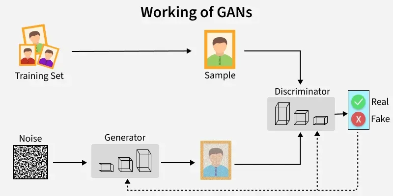
A Generative Adversarial Network, or GAN, consists of two neural networks:

  1. A generator \(G\),
  2. A discriminator \(D\).

Generative Adversarial Networks (GANs)

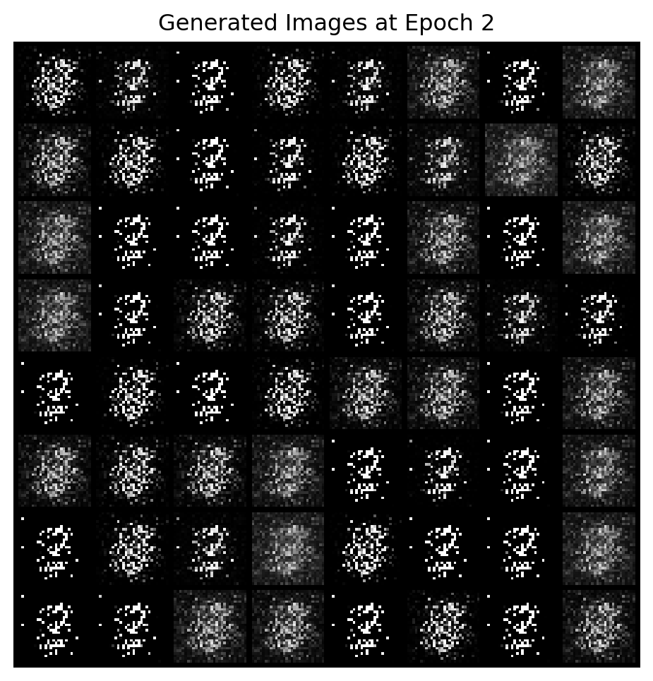
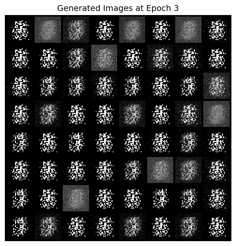
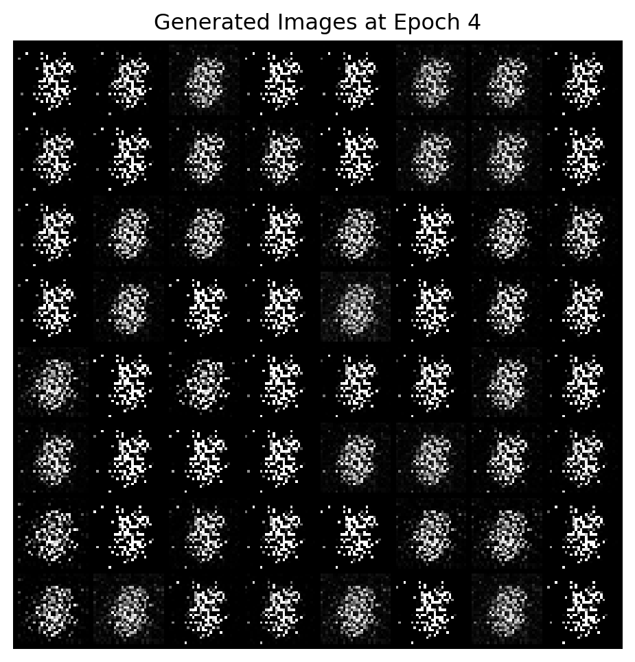
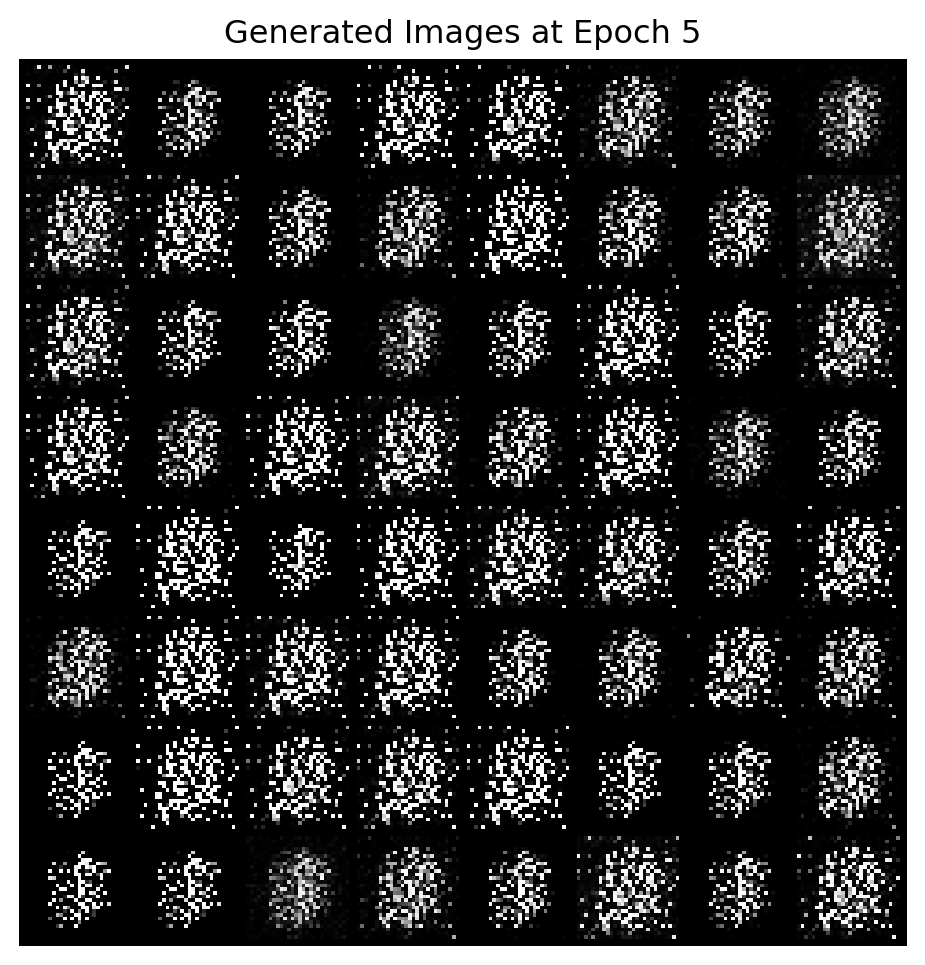
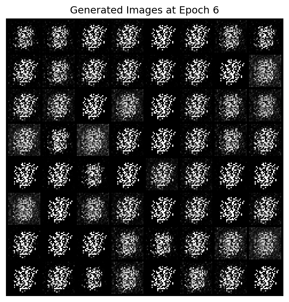
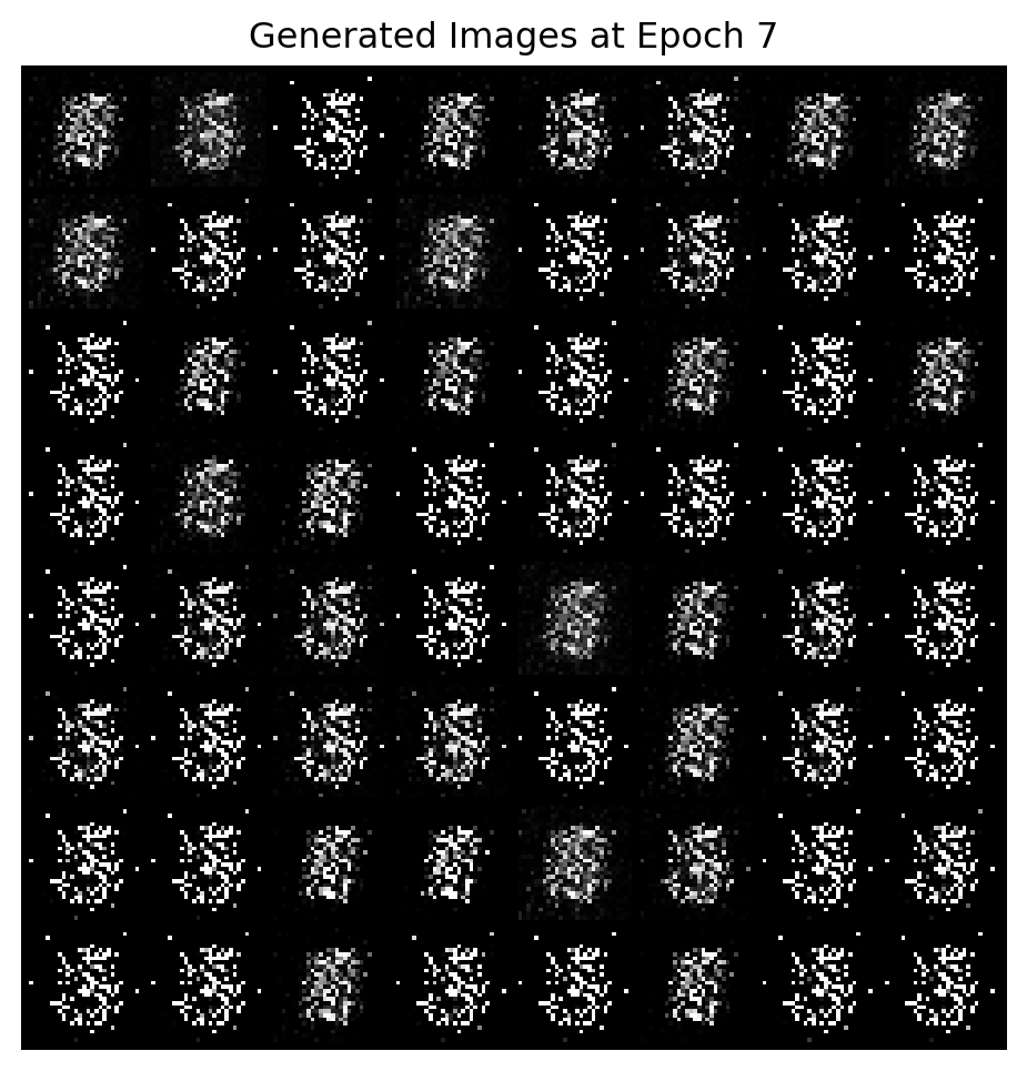
The generator maps random noise \(z\sim p_z\) to synthetic data \(G(z)\). The discriminator attempts to distinguish real data from generated data:

\[ D(x) \in (0, 1). \]

The classical GAN objective is

\[ \min_G \max_D \mathbb E_{x\sim P_{\text{data}}}[\log D(x) + \mathbb E_{z\sim p_x}[\log (1-D(G(z)))]]. \]

The discriminator tries to maximize this objective, while the generator tries to minimize it.

At idea equilibrium,

\[ p_g = p_\text{data}, \]

meaning the generator distribution matches the data distribution.

GANs are used for image synthesis, style transfer, data augmentation, and generative modeling, but they can be unstable to train.

Show code
# Simple GAN on MNIST
# pip install torch torchvision matplotlib

import torch
import torch.nn as nn
import torch.optim as optim
import matplotlib.pyplot as plt

from torchvision import datasets, transforms
from torch.utils.data import DataLoader
from torchvision.utils import make_grid

device = torch.device("cuda" if torch.cuda.is_available() else "cpu")

latent_dim = 100
image_dim = 28 * 28
batch_size = 128
epochs = 10
lr = 0.0002

transform = transforms.Compose([
    transforms.ToTensor(),
    transforms.Normalize((0.5,), (0.5,))   # scale images to [-1, 1]
])

dataset = datasets.MNIST(
    root="./data",
    train=True,
    transform=transform,
    download=True
)

loader = DataLoader(
    dataset,
    batch_size=batch_size,
    shuffle=True
)

class Generator(nn.Module):
    def __init__(self, latent_dim, image_dim):
        super().__init__()

        self.model = nn.Sequential(
            nn.Linear(latent_dim, 256),
            nn.LeakyReLU(0.2),

            nn.Linear(256, 512),
            nn.LeakyReLU(0.2),

            nn.Linear(512, 1024),
            nn.LeakyReLU(0.2),

            nn.Linear(1024, image_dim),
            nn.Tanh()   # output range [-1, 1]
        )

    def forward(self, z):
        return self.model(z)

class Discriminator(nn.Module):
    def __init__(self, image_dim):
        super().__init__()

        self.model = nn.Sequential(
            nn.Linear(image_dim, 512),
            nn.LeakyReLU(0.2),

            nn.Linear(512, 256),
            nn.LeakyReLU(0.2),

            nn.Linear(256, 1),
            nn.Sigmoid()   # probability real/fake
        )

    def forward(self, x):
        return self.model(x)


G = Generator(latent_dim, image_dim).to(device)
D = Discriminator(image_dim).to(device)

criterion = nn.BCELoss()

optimizer_G = optim.Adam(G.parameters(), lr=lr)
optimizer_D = optim.Adam(D.parameters(), lr=lr)


# Fixed noise so we can observe generator progress
fixed_noise = torch.randn(64, latent_dim).to(device)

def show_generated_images(generator, noise, epoch):
    generator.eval()

    with torch.no_grad():
        fake_images = generator(noise)
        fake_images = fake_images.view(-1, 1, 28, 28)

        # convert from [-1, 1] back to [0, 1]
        fake_images = (fake_images + 1) / 2

    grid = make_grid(fake_images, nrow=8)

    plt.figure(figsize=(6, 6))
    plt.imshow(grid.permute(1, 2, 0).cpu())
    plt.title(f"Generated Images at Epoch {epoch}")
    plt.axis("off")
    plt.show()

    generator.train()

for epoch in range(epochs):
    for real_images, _ in loader:
        real_images = real_images.view(-1, image_dim).to(device)

        current_batch_size = real_images.size(0)

        # Real labels = 1
        real_labels = torch.ones(current_batch_size, 1).to(device)

        # Fake labels = 0
        fake_labels = torch.zeros(current_batch_size, 1).to(device)
        
        # Train Discriminator
        # Real images
        real_outputs = D(real_images)
        d_loss_real = criterion(real_outputs, real_labels)

        # Fake images
        z = torch.randn(current_batch_size, latent_dim).to(device)
        fake_images = G(z)

        fake_outputs = D(fake_images.detach())
        d_loss_fake = criterion(fake_outputs, fake_labels)

        # Total discriminator loss
        d_loss = d_loss_real + d_loss_fake

        optimizer_D.zero_grad()
        d_loss.backward()
        optimizer_D.step()

        # Train Generator
        # Generator wants discriminator to think fake images are real
        z = torch.randn(current_batch_size, latent_dim).to(device)
        fake_images = G(z)

        outputs = D(fake_images)
        g_loss = criterion(outputs, real_labels)

        optimizer_G.zero_grad()
        g_loss.backward()
        optimizer_G.step()

    print(
        f"Epoch [{epoch + 1}/{epochs}] "
        f"D Loss: {d_loss.item():.4f} | "
        f"G Loss: {g_loss.item():.4f}"
    )

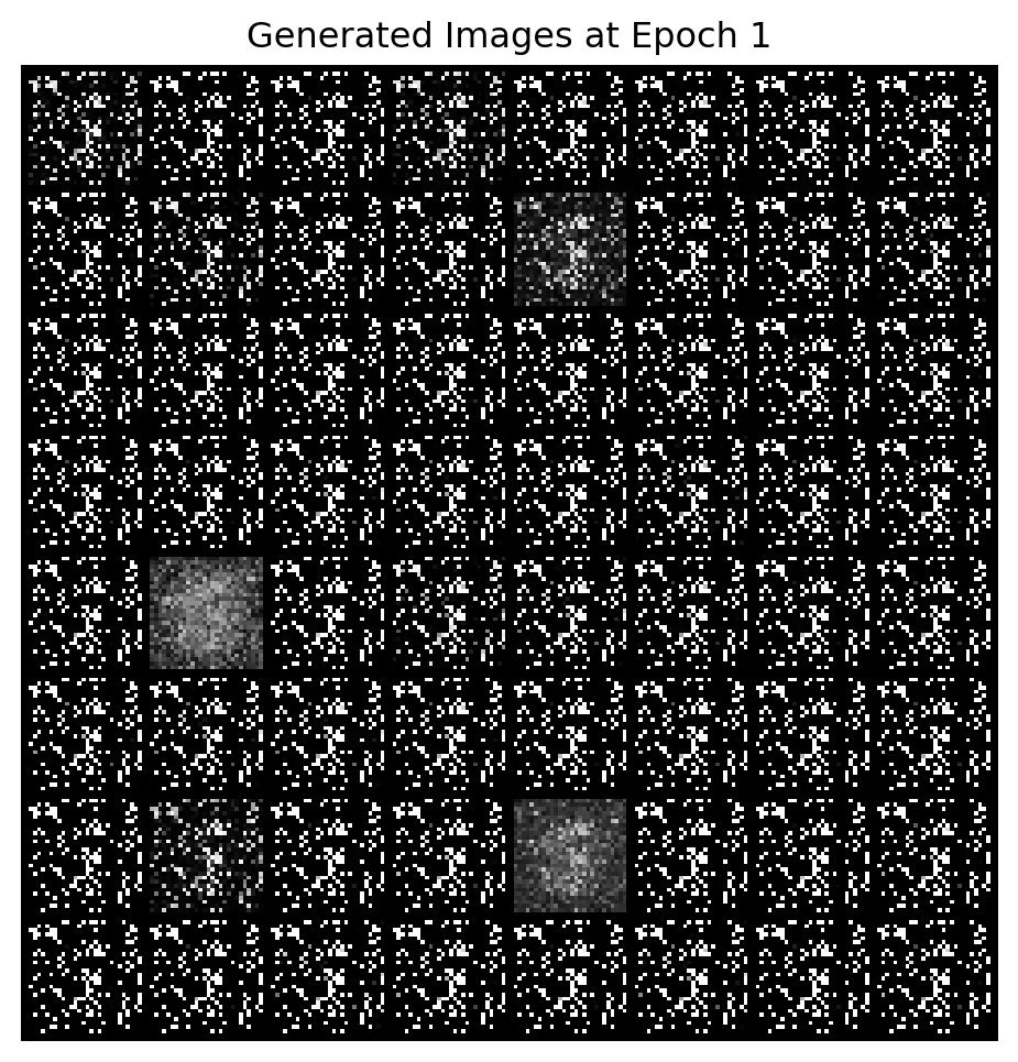
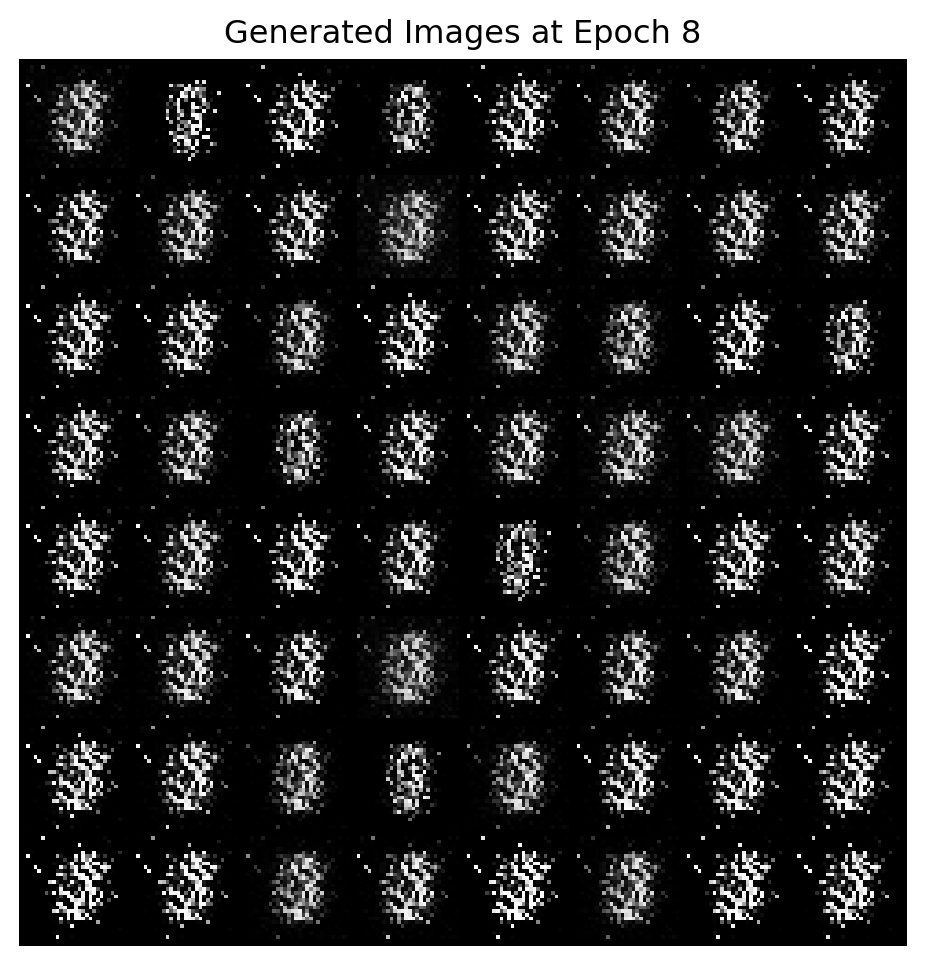
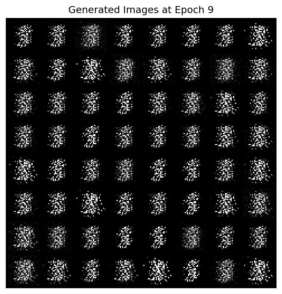
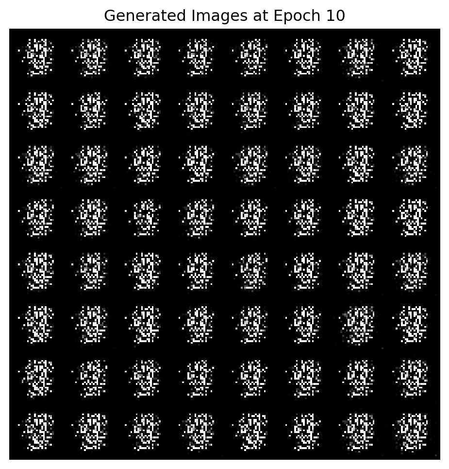
    show_generated_images(G, fixed_noise, epoch + 1)
Epoch [1/10] D Loss: 0.3123 | G Loss: 5.0729

Epoch [2/10] D Loss: 0.3735 | G Loss: 2.8431

Epoch [3/10] D Loss: 0.3441 | G Loss: 4.0207

Epoch [4/10] D Loss: 0.1579 | G Loss: 4.7931

Epoch [5/10] D Loss: 0.5683 | G Loss: 4.5528

Epoch [6/10] D Loss: 0.5326 | G Loss: 6.2303

Epoch [7/10] D Loss: 0.0825 | G Loss: 4.3888

Epoch [8/10] D Loss: 0.6070 | G Loss: 2.3785

Epoch [9/10] D Loss: 0.2869 | G Loss: 3.7709

Epoch [10/10] D Loss: 0.4038 | G Loss: 6.2876

8.7. Bayesian Neural Networks

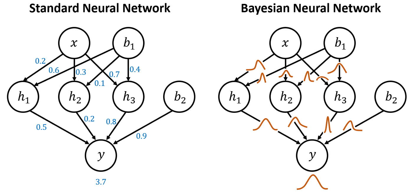
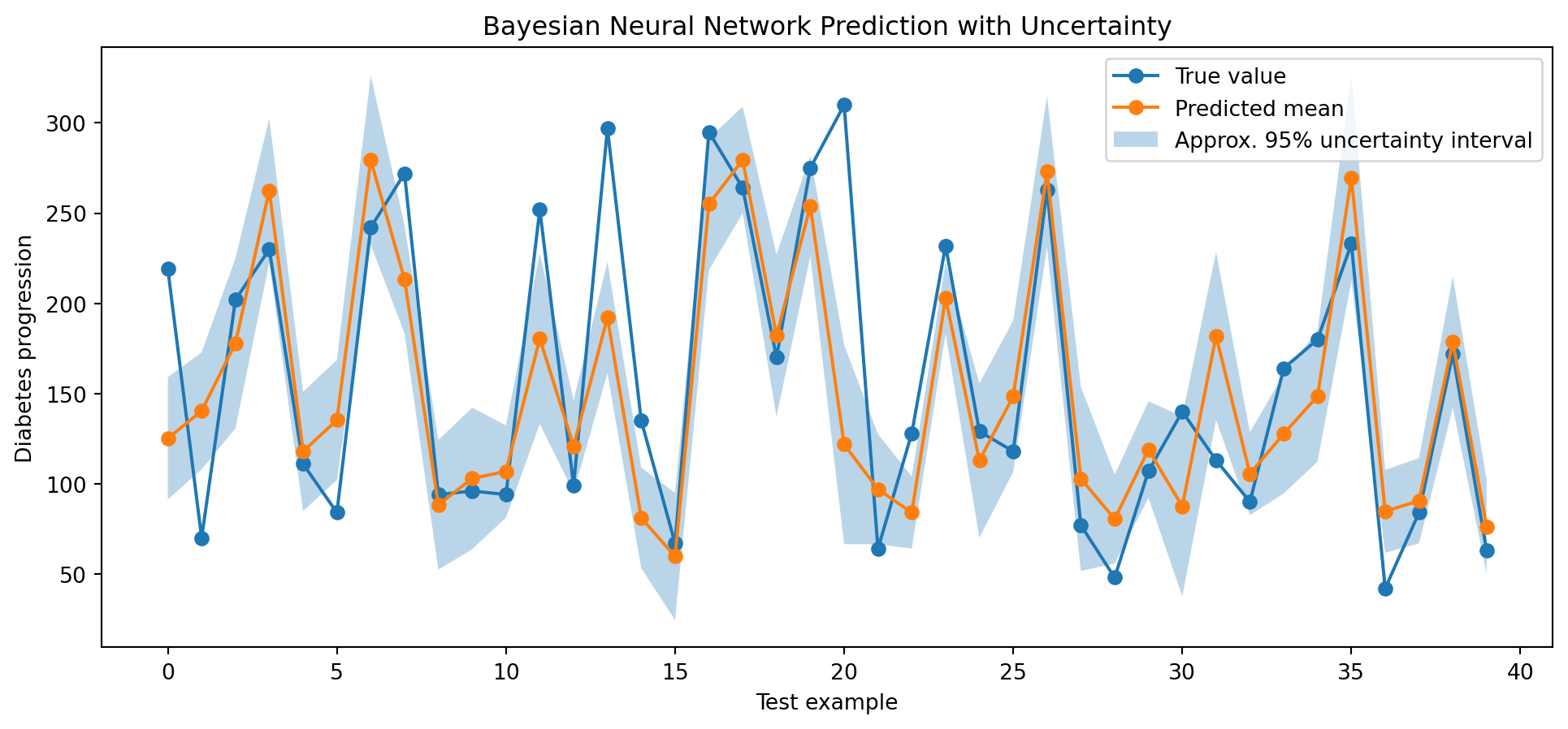
A Bayesian Neural Network places probability distributions over weights rather than treating weights as fixed unknown parameters.

Bayesian Neural Networks

Instead of estimating a single \(\theta\), we define a prior \(p(\theta)\) and compute a posterior

\[ p(\theta\,|\,\mathcal D)=\frac{p(\mathcal D\,|\, \theta)p(\theta)}{p(\mathcal D)}. \]

Predictions integrate over parameter uncertainty:

\[ p(y^*\,|\,x^*,\mathcal D) = \int p(y^*\,|\, x^*,\theta)p(\theta\,|\, \mathcal D)d\theta. \]

However, exact Bayesian inference in neural networks is usually intractable, so approximation methods such as variation inference, Monte Carlo dropout, Laplace approximations, or Markov chain Monte Carlo are used.

Show code
# Bayesian Neural Network idea using Monte Carlo Dropout
# Real example: diabetes progression prediction
#
# pip install torch scikit-learn matplotlib numpy

import numpy as np
import torch
import torch.nn as nn
import torch.optim as optim
import matplotlib.pyplot as plt

from sklearn.datasets import load_diabetes
from sklearn.model_selection import train_test_split
from sklearn.preprocessing import StandardScaler
from torch.utils.data import TensorDataset, DataLoader

np.random.seed(42)
torch.manual_seed(42)

data = load_diabetes()

X = data.data
y = data.target.reshape(-1, 1)

print("Feature names:", data.feature_names)
print("X shape:", X.shape)
print("y shape:", y.shape)

X_train, X_test, y_train, y_test = train_test_split(
    X,
    y,
    test_size=0.2,
    random_state=42
)


# Standardize features
x_scaler = StandardScaler()
X_train = x_scaler.fit_transform(X_train)
X_test = x_scaler.transform(X_test)


# Standardize target for easier neural network training
y_scaler = StandardScaler()
y_train_scaled = y_scaler.fit_transform(y_train)
y_test_scaled = y_scaler.transform(y_test)


# Convert to PyTorch tensors
X_train_tensor = torch.tensor(X_train, dtype=torch.float32)
y_train_tensor = torch.tensor(y_train_scaled, dtype=torch.float32)

X_test_tensor = torch.tensor(X_test, dtype=torch.float32)
y_test_tensor = torch.tensor(y_test_scaled, dtype=torch.float32)


train_dataset = TensorDataset(X_train_tensor, y_train_tensor)

train_loader = DataLoader(
    train_dataset,
    batch_size=32,
    shuffle=True
)

class MCDropoutBNN(nn.Module):
    def __init__(self, input_dim, dropout_rate=0.1):
        super().__init__()

        self.net = nn.Sequential(
            nn.Linear(input_dim, 64),
            nn.ReLU(),
            nn.Dropout(dropout_rate),

            nn.Linear(64, 64),
            nn.ReLU(),
            nn.Dropout(dropout_rate),

            nn.Linear(64, 1)
        )

    def forward(self, x):
        return self.net(x)


model = MCDropoutBNN(input_dim=X_train.shape[1], dropout_rate=0.1)

criterion = nn.MSELoss()
optimizer = optim.Adam(model.parameters(), lr=0.001)

epochs = 500

train_losses = []

for epoch in range(epochs):
    model.train()
    total_loss = 0

    for batch_X, batch_y in train_loader:
        preds = model(batch_X)

        loss = criterion(preds, batch_y)

        optimizer.zero_grad()
        loss.backward()
        optimizer.step()

        total_loss += loss.item()

    avg_loss = total_loss / len(train_loader)
    train_losses.append(avg_loss)

    if (epoch + 1) % 100 == 0:
        print(f"Epoch [{epoch + 1}/{epochs}], Loss: {avg_loss:.4f}")

plt.figure(figsize=(7, 4))
plt.plot(train_losses)
plt.title("Training Loss")
plt.xlabel("Epoch")
plt.ylabel("MSE Loss")
plt.show()
Feature names: ['age', 'sex', 'bmi', 'bp', 's1', 's2', 's3', 's4', 's5', 's6']
X shape: (442, 10)
y shape: (442, 1)
Epoch [100/500], Loss: 0.2927
Epoch [200/500], Loss: 0.2208
Epoch [300/500], Loss: 0.1904
Epoch [400/500], Loss: 0.1320
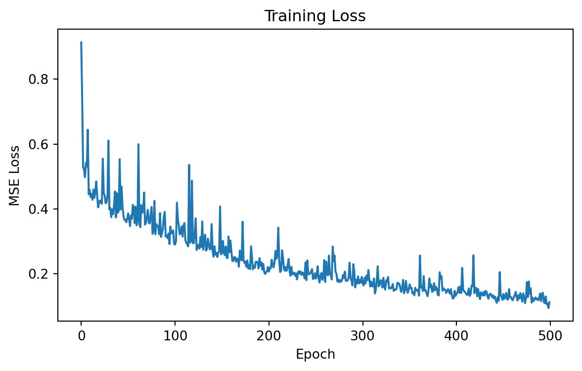
Epoch [500/500], Loss: 0.1126

Show code
# Monte Carlo Dropout prediction
def mc_dropout_predict(model, X, n_samples=200):
    """
    Runs the model many times with dropout ON.

    Returns:
    - mean prediction
    - prediction uncertainty
    - all sampled predictions
    """

    model.train()  
    # Important:
    # We use model.train() at test time so dropout remains active.

    predictions = []

    with torch.no_grad():
        for _ in range(n_samples):
            preds = model(X)
            predictions.append(preds.numpy())

    predictions = np.array(predictions)

    mean_prediction = predictions.mean(axis=0)
    uncertainty = predictions.std(axis=0)

    return mean_prediction, uncertainty, predictions


mean_scaled, uncertainty_scaled, all_predictions_scaled = mc_dropout_predict(
    model,
    X_test_tensor,
    n_samples=200
)


# Convert predictions back to original target scale
mean_prediction = y_scaler.inverse_transform(mean_scaled)
y_test_original = y_test

# For uncertainty, multiply by target standard deviation
uncertainty = uncertainty_scaled * y_scaler.scale_[0]
Show code
# Visualize prediction uncertainty
n_points = 40

true_values = y_test_original[:n_points].flatten()
predicted_values = mean_prediction[:n_points].flatten()
uncertainties = uncertainty[:n_points].flatten()

x_axis = np.arange(n_points)

plt.figure(figsize=(12, 5))

plt.plot(x_axis, true_values, marker="o", label="True value")
plt.plot(x_axis, predicted_values, marker="o", label="Predicted mean")

plt.fill_between(
    x_axis,
    predicted_values - 2 * uncertainties,
    predicted_values + 2 * uncertainties,
    alpha=0.3,
    label="Approx. 95% uncertainty interval"
)

plt.title("Bayesian Neural Network Prediction with Uncertainty")
plt.xlabel("Test example")
plt.ylabel("Diabetes progression")
plt.legend()
plt.show()

Show code
uncertainty_flat = uncertainty.flatten()
predicted_flat = mean_prediction.flatten()
true_flat = y_test_original.flatten()

most_uncertain_indices = np.argsort(uncertainty_flat)[-10:][::-1]

print("Most uncertain test examples:")
print()

for idx in most_uncertain_indices:
    print(
        f"Test index: {idx:3d} | "
        f"True: {true_flat[idx]:7.2f} | "
        f"Predicted: {predicted_flat[idx]:7.2f} | "
        f"Uncertainty: {uncertainty_flat[idx]:7.2f}"
    )
Most uncertain test examples:

Test index:  72 | True:  281.00 | Predicted:  290.00 | Uncertainty:   32.89
Test index:  75 | True:   91.00 | Predicted:  248.98 | Uncertainty:   29.69
Test index:  35 | True:  233.00 | Predicted:  269.68 | Uncertainty:   28.56
Test index:  79 | True:  233.00 | Predicted:  233.61 | Uncertainty:   28.29
Test index:  20 | True:  310.00 | Predicted:  121.79 | Uncertainty:   27.62
Test index:  68 | True:  140.00 | Predicted:  179.12 | Uncertainty:   25.89
Test index:  27 | True:   77.00 | Predicted:  102.81 | Uncertainty:   25.55
Test index:  70 | True:  101.00 | Predicted:   79.83 | Uncertainty:   25.19
Test index:  30 | True:  140.00 | Predicted:   87.49 | Uncertainty:   24.92
Test index:  54 | True:  171.00 | Predicted:  199.48 | Uncertainty:   24.76

9. Applications

9.1. Computer Vision

Neural networks, especially CNNs, are central to modern computer vision. Applications include:

  • handwritten digit recognition,
  • face authentication,
  • medication image diagnosis,
  • object detection,
  • image segmentation,
  • satellite image classification.

The typical image-classification mapping is

\[ f_\theta:\mathbb R^{H \times W\times C} \to \Delta^{K-1}, \]

where:

  • \(H, W, C\) is image height, width, and number of channels,
  • \(\Delta^{K-1}\) is the \(K\)-class probability simplex.

9.2. Natural Language Processing

In natural language processing, neural networks map sequences of tokens to predictions. A sequence is \(x=(x_1,x_2, \dots, x_T).\) Each token is embedded into a vector:

\[ e_t = E[x_t]. \]

The model then predicts outputs such as:

  • sentiment labels,
  • translated text,
  • named entitites,
  • summaries,
  • next-token probabilities.

For language modeling, the objective is often

\[ \max_{\theta}\sum_{t=1}^T \log P_\theta (x_t \,|\, x_1, \dots, x_{t-1}) \]

Equivalently, training minimizes negative log-likelihood:

\[ -\sum_{t=1}^T \log P_\theta(x_t\,|\, x_1,\dots, x_{t-1}) \]

9.3. Financial Services

In finance, neural networks are used for:

  • credit risk prediction,
  • fraud detection,
  • stock trend forecasting,
  • algorithmic trading,
  • customer segmentation.

For fraud detection, a neural network may estimate \(P(Y=\text{fraud}\,|\,x)\), where \(x\) includes transaction amount, location, merchant type, time, device, and user history.

9.4. Healthcare

In healthcare, neural networks are used for:

  • disease diagnosis,
  • medical image classification,
  • ECG arrhythmia detection,
  • drug discovery,
  • protein sequence classification.
  • patient outcome prediction

In high-stake settings, uncertainty and interpretability are critical. A model with high accuracy but poor calibration3 may be dangerous if clinicians interpret its output as a reliable probability.

9.5. Engineering and Control

Neural networks are used in:

  • robotics.
  • aircraft landing systems,
  • path planning,
  • energy management,
  • predictive maintenance.

In control settings, a neural network may approximate a policy \(\pi_\theta(a\,|\,s),\) where \(s\) is the system state and \(a\) is an action. The goal is to choose actions that optimize long-term reward.

9.6. Recommender Systems

Neural recommender systems learn embeddings for users and items.

Let \(u_i\in \mathbb R^d\) be a user embedding and \(v_j\in \mathbb R^d\) be an item embedding. A simple predicted preference score is

\[ \hat r_{ij} = u_i^\top v_j \]

More complex neural recommenders use nonlinear networks:

\[ \hat r_{ij} = f_\theta (u_i, v_j, \text{context}). \]

These models power personalized recommendations in video platforms, e-commerce, music services, and online advertising.

10. Black-Box Behavior and Interpretability

Neural networks are often called black-box models because their predictions result from many nested nonlinear transformations. A prediction may depend on millions or billions of parameters.

For a deep network \(f_\theta(x) = f^{(L)}\circ f^{(L-1)}\circ \cdots \circ f^{(1)}(x)\), even if every operation is mathematically explicit, the overall function can be difficult for humans to interpret.

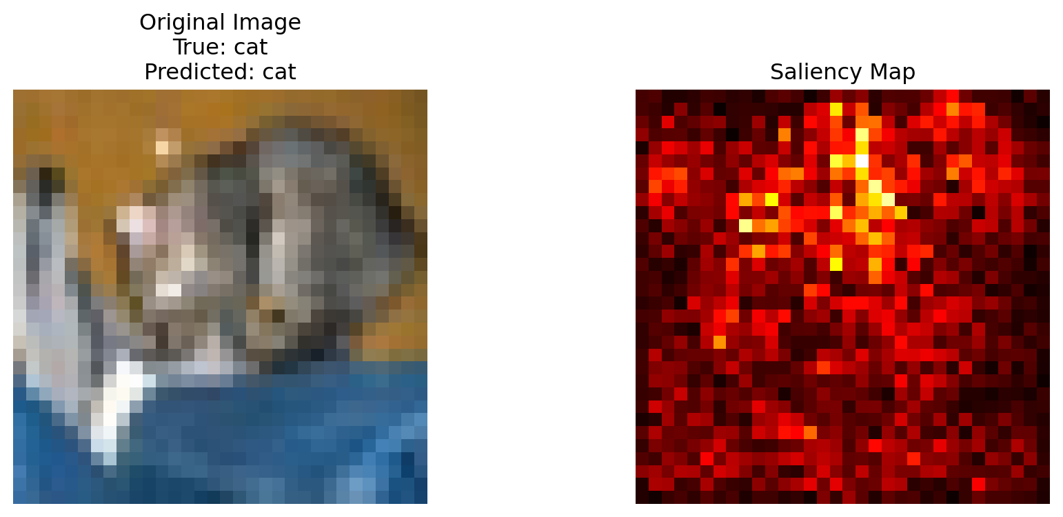
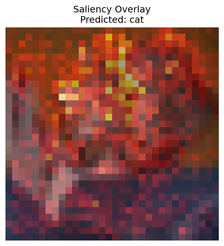
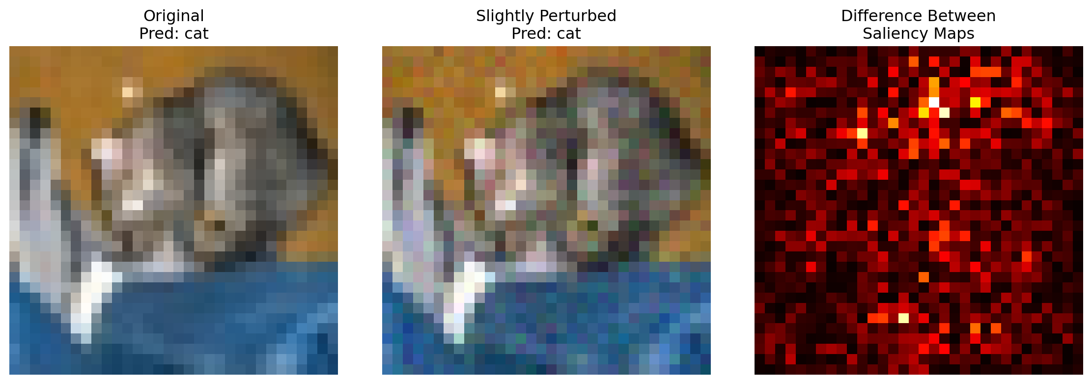
One mathematical way to examine sensitivity is the input gradient \(\nabla_x f_\theta(x)\). For image classification, a saliency map may use

\[ S_j(x) = \left|\frac{\partial f_\theta(x)}{\partial x_j}\right| \]

A large value of \(S_j(x)\) suggests that input feature \(j\) strongly influences the output locally. However, gradient-based explanations can be unstable and should not be treated as complete causal explanations.

Show code
# Saliency map example using CNN on CIFAR-10
# pip install torch torchvision matplotlib numpy

import torch
import torch.nn as nn
import torch.optim as optim
import matplotlib.pyplot as plt
import numpy as np

from torchvision import datasets, transforms
from torch.utils.data import DataLoader

device = torch.device("cuda" if torch.cuda.is_available() else "cpu")

batch_size = 128
epochs = 5
lr = 0.001

class_names = [
    "airplane", "automobile", "bird", "cat", "deer",
    "dog", "frog", "horse", "ship", "truck"
]

transform = transforms.Compose([
    transforms.ToTensor()
])

train_dataset = datasets.CIFAR10(
    root="./data",
    train=True,
    download=True,
    transform=transform
)

test_dataset = datasets.CIFAR10(
    root="./data",
    train=False,
    download=True,
    transform=transform
)

train_loader = DataLoader(
    train_dataset,
    batch_size=batch_size,
    shuffle=True
)

test_loader = DataLoader(
    test_dataset,
    batch_size=1,
    shuffle=False
)
Show code
class SimpleCIFARCNN(nn.Module):
    def __init__(self):
        super().__init__()

        self.features = nn.Sequential(
            nn.Conv2d(3, 32, kernel_size=3, padding=1),
            nn.ReLU(),
            nn.MaxPool2d(2),      # 32 x 16 x 16

            nn.Conv2d(32, 64, kernel_size=3, padding=1),
            nn.ReLU(),
            nn.MaxPool2d(2),      # 64 x 8 x 8

            nn.Conv2d(64, 128, kernel_size=3, padding=1),
            nn.ReLU(),
            nn.MaxPool2d(2)       # 128 x 4 x 4
        )

        self.classifier = nn.Sequential(
            nn.Flatten(),
            nn.Linear(128 * 4 * 4, 256),
            nn.ReLU(),
            nn.Linear(256, 10)
        )

    def forward(self, x):
        x = self.features(x)
        x = self.classifier(x)
        return x


model = SimpleCIFARCNN().to(device)
Show code
criterion = nn.CrossEntropyLoss()
optimizer = optim.Adam(model.parameters(), lr=lr)

for epoch in range(epochs):
    model.train()
    total_loss = 0
    correct = 0
    total = 0

    for images, labels in train_loader:
        images = images.to(device)
        labels = labels.to(device)

        logits = model(images)
        loss = criterion(logits, labels)

        optimizer.zero_grad()
        loss.backward()
        optimizer.step()

        total_loss += loss.item()

        preds = logits.argmax(dim=1)
        correct += (preds == labels).sum().item()
        total += labels.size(0)

    avg_loss = total_loss / len(train_loader)
    accuracy = correct / total

    print(
        f"Epoch [{epoch + 1}/{epochs}] "
        f"Loss: {avg_loss:.4f} | "
        f"Train Accuracy: {accuracy:.4f}"
    )
Epoch [1/5] Loss: 1.5987 | Train Accuracy: 0.4108
Epoch [2/5] Loss: 1.2199 | Train Accuracy: 0.5637
Epoch [3/5] Loss: 1.0391 | Train Accuracy: 0.6318
Epoch [4/5] Loss: 0.9013 | Train Accuracy: 0.6853
Epoch [5/5] Loss: 0.7996 | Train Accuracy: 0.7192
Show code
def compute_saliency(model, image, target_class=None):
    """
    image shape: [1, 3, 32, 32]

    Returns:
    - predicted class
    - RGB saliency map
    - grayscale saliency map
    """

    model.eval()

    # We want gradient with respect to the input image
    image = image.clone().detach().to(device)
    image.requires_grad = True

    logits = model(image)

    predicted_class = logits.argmax(dim=1).item()

    if target_class is None:
        target_class = predicted_class

    # The score for the chosen class
    score = logits[0, target_class]

    model.zero_grad()
    score.backward()

    # Gradient shape: [1, 3, 32, 32]
    saliency_rgb = image.grad.abs().squeeze().detach().cpu()

    # Combine RGB channels into one map
    saliency_gray = saliency_rgb.max(dim=0)[0]

    return predicted_class, saliency_rgb, saliency_gray
Show code
image, true_label = next(iter(test_loader))

predicted_class, saliency_rgb, saliency_gray = compute_saliency(model, image)

original_image = image.squeeze().permute(1, 2, 0).detach().cpu()

plt.figure(figsize=(10, 4))

plt.subplot(1, 2, 1)
plt.imshow(original_image)
plt.title(
    f"Original Image\n"
    f"True: {class_names[true_label.item()]}\n"
    f"Predicted: {class_names[predicted_class]}"
)
plt.axis("off")

plt.subplot(1, 2, 2)
plt.imshow(saliency_gray, cmap="hot")
plt.title("Saliency Map")
plt.axis("off")

plt.tight_layout()
plt.show()

Show code
plt.figure(figsize=(5, 5))

plt.imshow(original_image)
plt.imshow(saliency_gray, cmap="hot", alpha=0.5)

plt.title(
    f"Saliency Overlay\n"
    f"Predicted: {class_names[predicted_class]}"
)
plt.axis("off")

plt.show()

Show code
noise = 0.03 * torch.randn_like(image)
perturbed_image = torch.clamp(image + noise, 0, 1)

pred_original, _, saliency_original = compute_saliency(model, image)
pred_perturbed, _, saliency_perturbed = compute_saliency(model, perturbed_image)

difference = torch.abs(saliency_original - saliency_perturbed)

plt.figure(figsize=(12, 4))

plt.subplot(1, 3, 1)
plt.imshow(image.squeeze().permute(1, 2, 0).detach().cpu())
plt.title(f"Original\nPred: {class_names[pred_original]}")
plt.axis("off")

plt.subplot(1, 3, 2)
plt.imshow(perturbed_image.squeeze().permute(1, 2, 0).detach().cpu())
plt.title(f"Slightly Perturbed\nPred: {class_names[pred_perturbed]}")
plt.axis("off")

plt.subplot(1, 3, 3)
plt.imshow(difference, cmap="hot")
plt.title("Difference Between\nSaliency Maps")
plt.axis("off")

plt.tight_layout()
plt.show()


Artificial Neural Networks are nonlinear, compositional function approximators. Their basic computational unit is simple: a weighted sum, a bias, and an activation function. Their power comes from composing many such units into layered architectures capable of learning complex representations.

The multilayer perceptron provides the foundation. A network maps inputs through repeated transformations

\[ z^{(\ell)}=W^{(\ell)}a^{(\ell-1)}+b^{(\ell)},
\qquad
a^{(\ell)}=\sigma(z^{(\ell)}). \] Training minimizes a loss function using backpropagation, which efficiently computes gradients through the chain rule. The central backpropagation recursion,

\[ \delta^{(\ell)}
=
((W^{(\ell+1)})^\top\delta^{(\ell+1)})
\odot
\sigma'(z^{(\ell)}), \] explains how errors move backward through the network and how weights are updated.

Neural networks are expressive enough to approximate broad classes of functions, but this expressive power creates practical challenges: nonconvex optimization, overfitting, vanishing gradients, hyperparameter sensitivity, computational cost, and weak interpretability. Regularization methods such as weight decay, dropout, and early stopping help control generalization.

Modern neural architectures extend the basic ANN idea to specialized data structures. CNNs exploit spatial locality in images. RNNs and LSTMs model sequences. Transformers use attention to model global dependencies. Autoencoders learn compressed representations. GANs generate synthetic data through adversarial training. Bayesian neural networks represent uncertainty by treating weights probabilistically.

Next chapter: Data modeling - Bayesian Inference

Footnotes

  1. Rumelhart, David E., Geoffrey E. Hinton, and Ronald J. Williams. “Learning Representations by Back-Propagating Errors.” Nature 323, no. 6088 (1986): 533–36. https://doi.org/10.1038/323533a0.↩︎
  2. Cybenko, G. “Approximation by Superpositions of a Sigmoidal Function.” Mathematics of Control, Signals and Systems 2, no. 4 (1989): 303–14. https://doi.org/10.1007/BF02551274.↩︎
  3. For a predicted probability, \(\hat p = P(Y=1\,|\, x)\), calibration means that among cases assigned probability 0.8, about 80% should truly belong to the positive class.↩︎