Debugging and Evaluating

The preceding chapters developed mathematical models for regression, classification, dimensionality reduction, clustering, Bayesian inference, and nonlinear representation learning. Those methods may produce elegant equations, low optimization loss, and impressive validation scores. None of these achievements alone establishes that a model is useful.

A model becomes valuable only when it performs reliably on observations that were not used to construct it, supports a meaningful decision, remains stable under realistic operating conditions, and produces benefits greater than its practical costs.

In research, the model is often treated as the principal object. In deployment, the model is only one component of a larger system involving:

• data collection;
• feature computation;
• software pipelines;
• decision thresholds;
• human review;
• monitoring;
• retraining;
• security;
• governance;
• operational costs;
• consequences of incorrect decisions.

Production machine-learning systems can accumulate failure modes beyond ordinary software defects because their behavior depends on changing data and on interactions among many data-producing and data-consuming components. This creates forms of technical debt that may not be visible from an offline accuracy score alone¹.

The central principle of this chapter is:

A model is not evaluated by asking only whether it predicts accurately. It is evaluated by asking whether it makes the intended decision better, under the conditions in which it will actually operate.

The practical evaluation process therefore asks five questions:

1. Validity: Was the model evaluated without leakage or contamination?
2. Generalization: Does it work on genuinely unseen and representative data?
3. Decision value: Does it improve the action that stakeholders care about?
4. Robustness: Does it remain reliable under perturbation, subgroup variation, and distribution shift?
5. Operational readiness: Can it be monitored, maintained, reproduced, and safely replaced?

1. Evaluation as a Decision Problem

1.1. Prediction Quality is Not the Final Objective

Suppose a model predicts whether a customer will cancel a subscription. A data scientist may report \(\operatorname{AUC}=0.86\). A stakeholder may instead ask:

• How many customers should receive a retention offer?
• How much does each offer cost?
• How many cancellations can realistically be prevented?
• What happens if loyal customers receive unnecessary discounts?
• Is the campaign more profitable than the existing strategy?
• Can the marketing team contact the selected customers in time?

The model score is only an intermediate quantity. The final quantity is often an expected operational value.

Let:

• \(a\in\mathcal A\) denote an action;
• \(Y\) denote an uncertain outcome;
• \(U(a,Y)\) denote the utility or financial value of action a when outcome Y occurs;
• \(x\) denote available information.

The decision rule should ideally choose

\[ a^*(x) = \arg\max_{a\in\mathcal A} \mathbb E[U(a,Y)\mid X=x]. \]

A predictive model estimates information required by this decision. It does not define the utility function.

This distinction is essential. Two models with similar statistical performance can produce very different operational value if their errors occur in different cases or if they are used with different thresholds.

1.2. The Cost Matrix

For binary classification, let the positive class represent an event such as fraud, disease, equipment failure, or customer cancellation.

A decision produces one of four outcomes:

Actual outcome	Predicted positive	Predicted negative
Positive	True positive	False negative
Negative	False positive	True negative

Assign costs

\[ C_{\mathrm{TP}}, \quad C_{\mathrm{FP}}, \quad C_{\mathrm{FN}}, \quad C_{\mathrm{TN}}. \]

The total cost is

\[ C_{\text{total}} = C_{\mathrm{TP}}TP + C_{\mathrm{FP}}FP + C_{\mathrm{FN}}FN + C_{\mathrm{TN}}TN. \]

Frequently,

\[ C_{\mathrm{FN}}\neq C_{\mathrm{FP}}. \]

For example:

• In cancer screening, a false negative may delay treatment.
• In fraud prevention, a false positive may block a legitimate customer.
• In spam filtering, a false positive may hide an important message.
• In predictive maintenance, a false negative may cause equipment damage, while a false positive may cause unnecessary inspection.

Accuracy treats every mistake equally:

\[ \operatorname{Accuracy} = \frac{TP+TN}{TP+TN+FP+FN}. \]

Real decisions rarely do.

1.3. Deriving a Decision Threshold from Costs

Suppose a calibrated model estimates

\[ p(x)=P(Y=1\mid X=x). \]

Consider two actions:

• predict or act positive;
• predict or act negative.

Assume zero cost for correct decisions for simplicity. The expected cost of predicting positive is

\[ R(+\mid x) = C_{\mathrm{FP}}P(Y=0\mid x) = C_{\mathrm{FP}}(1-p(x)). \]

The expected cost of predicting negative is

\[ R(-\mid x) = C_{\mathrm{FN}}P(Y=1\mid x) = C_{\mathrm{FN}}p(x). \]

Choose the positive action when

\[ R(+\mid x)<R(-\mid x). \]

Therefore,

\[ C_{\mathrm{FP}}(1-p) < C_{\mathrm{FN}}p. \]

Rearranging,

\[ C_{\mathrm{FP}} < p(C_{\mathrm{FP}}+C_{\mathrm{FN}}), \]

so the optimal threshold is

\[ p(x) > \frac{C_{\mathrm{FP}}} {C_{\mathrm{FP}}+C_{\mathrm{FN}}}. \]

Thus, the conventional threshold 0.5 is optimal only under particular cost assumptions. If false negatives are much more costly than false positives, the appropriate threshold can be substantially below 0.5.

1.4. Stakeholder Metrics

A useful evaluation translates statistical quantities into operational language.

Instead of reporting only \(\operatorname{Recall}=0.82\), report:

At the selected operating threshold, the system identifies approximately 82 of every 100 actual failures, while generating 14 unnecessary inspections per 1,000 machines.

Instead of reporting only \(RMSE=12.4\), report:

The typical error is approximately 12 units, but for the highest-value accounts it rises to 31 units.

Instead of reporting only \(\operatorname{AUC}=0.91\), report:

If one fraud case and one legitimate transaction are selected at random, the model ranks the fraud case higher approximately 91% of the time.

The stakeholder normally cares about:

• dollars gained or lost;
• failures prevented;
• patients missed;
• cases requiring manual review;
• time saved;
• service-level constraints;
• capacity limits;
• downstream harms.

The evaluation should be built around those quantities.

2. Designing a Trustworthy Evaluation

2.1. Training, Validation, and Test Data

Let the available dataset be \(D=\{(x_i,y_i)\}_{i=1}^{N}\).

A standard partition contains:

• training data \(D_{\mathrm{train}}\);
• validation data \(D_{\mathrm{val}}\);
• test data \(D_{\mathrm{test}}\).

The training set estimates model parameters. The validation set selects:

• model family;
• hyperparameters;
• feature transformations;
• decision thresholds;
• regularization strength;
• stopping time.

The test set estimates performance only after the full modeling procedure has been selected.

The test data should be treated as a sealed evaluation resource. If the researcher repeatedly checks test performance and modifies the model in response, the test set becomes another validation set.

The final evaluation must test the whole procedure, not only the final mathematical estimator.

2.2. The Evaluation Unit Must Match Deployment

A random row-level split is not always valid.

Suppose a hospital dataset contains several visits per patient. If visits from the same patient appear in both training and test sets, the model may exploit patient-specific information that will not be available when predicting for a genuinely new patient.

Possible split units include:

• patient;
• household;
• customer;
• device;
• geographic region;
• school;
• company;
• time period;
• document source.

The grouping unit should match the unit over which generalization is claimed.

If the deployment goal is prediction for future visits of existing patients, a patient-overlapping temporal split may be reasonable. If the goal is prediction for new patients, patients must not overlap.

2.3. Random, Grouped, Spatial, and Temporal Splits

2.3.1. Random split

A random split is suitable when observations are approximately independent and exchangeable:

\[ (X_i,Y_i) \overset{\text{i.i.d.}}{\sim} P. \]

2.3.2. Stratified split

For rare classes, stratification approximately preserves class proportions in each partition.

2.3.3. Grouped split

All observations from the same group are assigned together:

\[ g_i=g_j \implies \operatorname{split}(i)=\operatorname{split}(j). \]

2.3.4. Temporal split

Training observations precede test observations:

\[ t_i<t_j \quad \text{for training }i \text{ and test }j. \]

This imitates forecasting deployment and prevents future information from influencing past predictions.

2.3.5. Spatial split

Geographic regions are separated to evaluate transfer to new locations.

A spatial model tested by randomly splitting nearby observations may benefit from strong spatial autocorrelation and provide an optimistic estimate of performance at genuinely new sites.

2.4. Cross-Validation

In K-fold cross-validation, the development data are partitioned into folds \(F_1,\ldots,F_K\).

For each fold \(k\), train the full modeling procedure on \(D\setminus F_k\) and evaluate on \(F_k\).

For loss function L, the estimate is

\[ \widehat R_{\mathrm{CV}} = \frac1N \sum_{k=1}^{K} \sum_{i\in F_k} L \left( y_i, \hat f^{(-k)}(x_i) \right). \]

Cross-validation is useful both for model selection and for estimating performance.

2.5. Nested Cross-Validation

Suppose hyperparameters are selected by minimizing cross-validation error:

\[ \hat\lambda = \arg\min_{\lambda\in\Lambda} \widehat R_{\mathrm{CV}}(\lambda). \]

Reporting the same minimum error

\[ \min_{\lambda\in\Lambda} \widehat R_{\mathrm{CV}}(\lambda) \]

is optimistic because the estimate was used to choose \(\lambda\).

Nested cross-validation separates tuning from evaluation:

• the inner loop selects hyperparameters;
• the outer loop evaluates the complete selection procedure.

For outer folds \(G_1,\ldots,G_J\):

1. Reserve \(G_j\) as the outer test fold.
2. Use only \(D\setminus G_j\) to tune the model through inner cross-validation.
3. Refit the selected procedure on \(D\setminus G_j\).
4. Evaluate on \(G_j\).
5. Aggregate the outer-fold losses.

This evaluates what would happen if the entire model-selection process were repeated on new data.

2.6. Data Leakage

NoteDefinition 1: Data Leakage

Data leakage occurs when model training or model selection uses information that would not be available at the time of prediction or that belongs to the evaluation observations.

Leakage can enter through:

• scaling before splitting;
• imputation using all observations;
• feature selection using the full dataset;
• PCA before cross-validation;
• target-derived features;
• future timestamps;
• duplicate observations;
• patient overlap;
• post-outcome variables;
• manual corrections informed by test labels;
• threshold selection on test data.

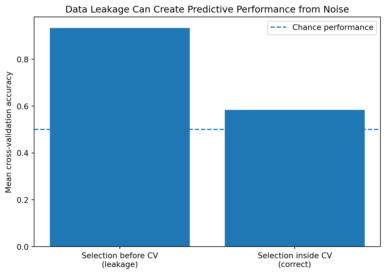
Leakage can produce apparently excellent performance even when no real predictive relationship exists.

import numpy as np
import matplotlib.pyplot as plt

from sklearn.feature_selection import SelectKBest, f_classif
from sklearn.linear_model import LogisticRegression
from sklearn.model_selection import StratifiedKFold, cross_val_score
from sklearn.pipeline import Pipeline
from sklearn.preprocessing import StandardScaler

rng = np.random.default_rng(42)

n_observations = 120
n_features = 5000

X = rng.normal(size=(n_observations, n_features))
y = rng.integers(0, 2, size=n_observations)

cv = StratifiedKFold(
    n_splits=5,
    shuffle=True,
    random_state=42
)

# Wrong: feature selection sees every label before cross-validation.
selector = SelectKBest(f_classif, k=20)
X_leaked = selector.fit_transform(X, y)

leaked_model = Pipeline([
    ("scaler", StandardScaler()),
    ("classifier", LogisticRegression(max_iter=3000))
])

leaked_scores = cross_val_score(
    leaked_model,
    X_leaked,
    y,
    cv=cv,
    scoring="accuracy"
)

# Correct: selection is fitted only on each training fold.
correct_model = Pipeline([
    ("selector", SelectKBest(f_classif, k=20)),
    ("scaler", StandardScaler()),
    ("classifier", LogisticRegression(max_iter=3000))
])

correct_scores = cross_val_score(
    correct_model,
    X,
    y,
    cv=cv,
    scoring="accuracy"
)

results = [
    leaked_scores.mean(),
    correct_scores.mean()
]

plt.figure(figsize=(7, 5))
plt.bar(
    ["Selection before CV\n(leakage)", "Selection inside CV\n(correct)"],
    results
)
plt.axhline(
    0.5,
    linestyle="--",
    label="Chance performance"
)
plt.ylabel("Mean cross-validation accuracy")
plt.title("Data Leakage Can Create Predictive Performance from Noise")
plt.legend()
plt.tight_layout()
plt.show()

print("Leaked scores:", leaked_scores)
print("Correct scores:", correct_scores)

Leaked scores: [1.         0.91666667 0.91666667 0.91666667 0.91666667]
Correct scores: [0.625      0.5        0.625      0.58333333 0.58333333]

2.7. Bootstrap Evaluation

A bootstrap sample draws \(N\) observations with replacement from the original sample. Some observations appear multiple times, while others are omitted.

The probability that a particular observation is absent is

\[ \left(1-\frac1N\right)^N \rightarrow e^{-1} \approx0.368. \]

Therefore, approximately \(1-e^{-1}\approx0.632\) of distinct observations appear in an ordinary bootstrap sample.

The original \(.632\) estimator combines apparent training error and out-of-bootstrap error:

\[ \widehat R_{.632} = 0.368\widehat R_{\mathrm{train}} + 0.632\widehat R_{\mathrm{OOB}}. \]

The .632+ estimator modifies the weight to address severe overfitting. Efron and Tibshirani developed the .632+ method as an improvement for estimating prediction error in overfit settings².

Bootstrap evaluation is especially useful for:

• uncertainty intervals;
• optimism correction;
• small datasets;
• assessing coefficient stability;
• comparing model variability.

3. Bias, Variance, and Learning Curves

3.1. Bias–Variance Decomposition

Assume \(Y=f(X)+\varepsilon\),

where

\[ \mathbb E[\varepsilon\mid X]=0, \qquad \operatorname{Var}(\varepsilon\mid X=x)=\sigma^2. \]

Let \(\hat f_D(x)\) denote a model trained on random dataset \(D\).

At a fixed input \(x\),

\[ \mathbb E_D \mathbb E_{Y\mid x} \left[ (Y-\hat f_D(x))^2 \right] \]

decomposes as

\[ \sigma^2 + \left( \mathbb E_D[\hat f_D(x)]-f(x) \right)^2 + \operatorname{Var}_D(\hat f_D(x)). \]

These terms are:

\[ \text{irreducible noise} + \text{squared bias} + \text{variance}. \]

TipDerivation

Write

\[ Y-\hat f_D(x) = \varepsilon + f(x)-\hat f_D(x). \]

Squaring and taking expectations removes the cross-term because

\[ \mathbb E[\varepsilon\mid X=x]=0. \]

Then insert and subtract

\[ \bar f(x) = \mathbb E_D[\hat f_D(x)]. \]

The expected squared deviation separates into

\[ (f(x)-\bar f(x))^2 + \mathbb E_D[ (\hat f_D(x)-\bar f(x))^2 ]. \]

These are squared bias and variance.

3.2. Practical Signs of Bias and Variance

High bias

• training performance is poor;
• validation performance is similarly poor;
• residual patterns remain systematic;
• adding more data produces little improvement;
• increasing model flexibility may help.

High variance

• training performance is excellent;
• validation performance is substantially worse;
• results vary across folds or random seeds;
• coefficients or selected features are unstable;
• more data or stronger regularization may help.

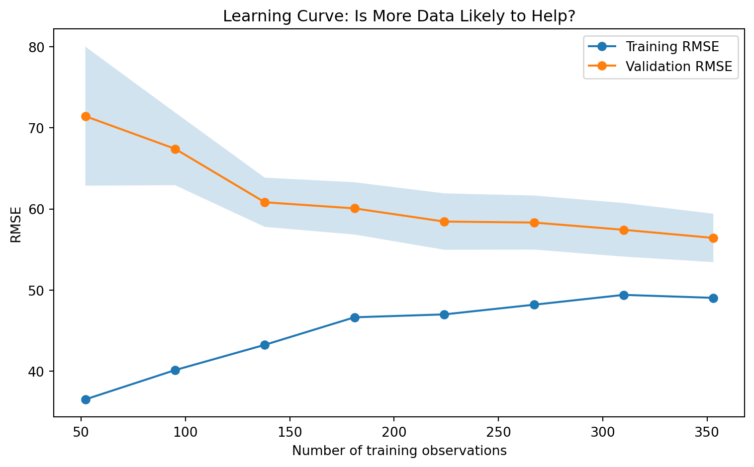
Data limitation

• training and validation performance are both improving as data increase;
• the learning curve has not plateaued;
• acquiring additional representative data may be more valuable than changing algorithms.

3.3. Learning Curves

A learning curve plots performance against training-set size.

Let \(m_1<m_2<\cdots<m_R\) be sample sizes. For each \(m_r\):

1. draw or select a training sample of size \(m_r\);
2. fit the model;
3. record training and validation loss;
4. repeat to measure variability.

import numpy as np
import matplotlib.pyplot as plt

from sklearn.datasets import load_diabetes
from sklearn.model_selection import learning_curve, KFold
from sklearn.pipeline import Pipeline
from sklearn.preprocessing import StandardScaler, PolynomialFeatures
from sklearn.linear_model import Ridge

data = load_diabetes()
X = data.data
y = data.target

model = Pipeline([
    ("polynomial", PolynomialFeatures(
        degree=2,
        include_bias=False
    )),
    ("scaler", StandardScaler()),
    ("ridge", Ridge(alpha=10.0))
])

cv = KFold(
    n_splits=5,
    shuffle=True,
    random_state=42
)

sizes, train_scores, validation_scores = learning_curve(
    model,
    X,
    y,
    train_sizes=np.linspace(0.15, 1.0, 8),
    cv=cv,
    scoring="neg_root_mean_squared_error"
)

train_rmse = -train_scores.mean(axis=1)
validation_rmse = -validation_scores.mean(axis=1)
validation_std = validation_scores.std(axis=1)

plt.figure(figsize=(8, 5))
plt.plot(sizes, train_rmse, marker="o", label="Training RMSE")
plt.plot(
    sizes,
    validation_rmse,
    marker="o",
    label="Validation RMSE"
)
plt.fill_between(
    sizes,
    validation_rmse - validation_std,
    validation_rmse + validation_std,
    alpha=0.2
)
plt.title("Learning Curve: Is More Data Likely to Help?")
plt.xlabel("Number of training observations")
plt.ylabel("RMSE")
plt.legend()
plt.tight_layout()
plt.show()

4. Regression Evaluation and Debugging

4.1. Regression Metrics

Let residuals be \(e_i=y_i-\hat y_i\).

Mean squared error

\[ MSE = \frac1N \sum_{i=1}^{N}e_i^2. \]

MSE corresponds to the mean negative log-likelihood under a homoskedastic Gaussian error model, apart from constants and scale.

Root mean squared error

\[ RMSE=\sqrt{MSE}. \]

RMSE has the same units as the response.

Mean absolute error

\[ MAE = \frac1N \sum_{i=1}^{N}|e_i|. \]

MAE is less dominated by large residuals than RMSE.

Median absolute error

\[ \operatorname{MedAE} = \operatorname{median}_i|e_i|. \]

This describes a typical absolute error robustly.

Coefficient of determination

\[ R^2 = 1- \frac{ \sum_i(y_i-\hat y_i)^2 }{ \sum_i(y_i-\bar y)^2 }. \]

On unseen data, \(R^2\) can be negative. This means the model performs worse than the baseline that predicts the test-set mean under the corresponding definition.

4.2. Choosing Between MAE and RMSE

RMSE penalizes large errors more strongly because \(e^2\) grows faster than \(|e|\).

If an error of 20 is more than twice as harmful as an error of 10, RMSE may align better with the decision.

If cost grows approximately linearly with error, MAE may be more suitable.

The chosen metric should reflect operational cost, not convention.

For example:

• electricity imbalance penalties may rise sharply for large misses;
• delivery-time error may be approximately linear;
• financial loss may be asymmetric;
• underprediction and overprediction may have different costs.

An asymmetric loss can be written as

\[ L_\tau(y,\hat y) = \begin{cases} \tau(y-\hat y), & y\geq\hat y,\\ (1-\tau)(\hat y-y), & y<\hat y. \end{cases} \]

This is the quantile or pinball loss.

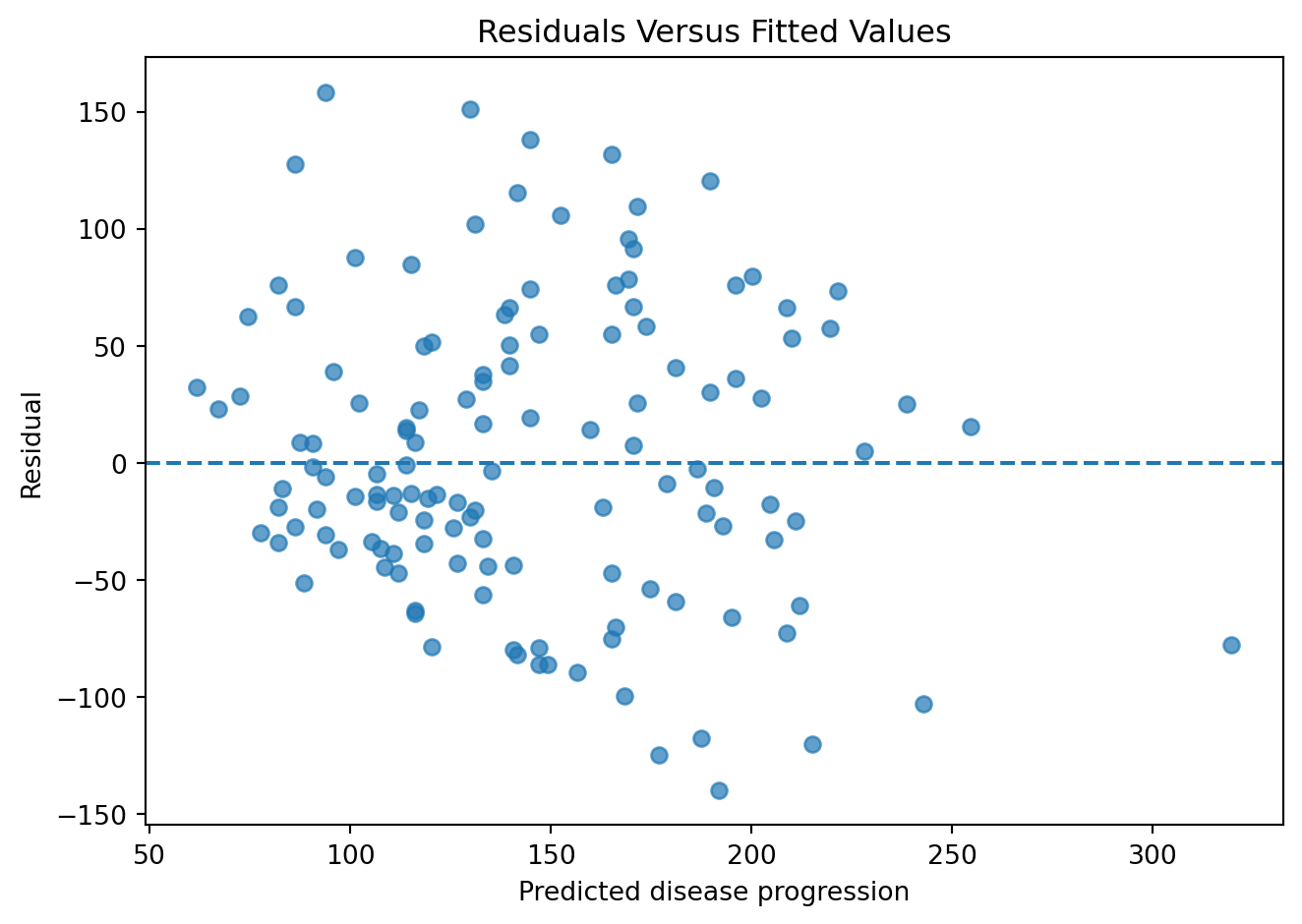
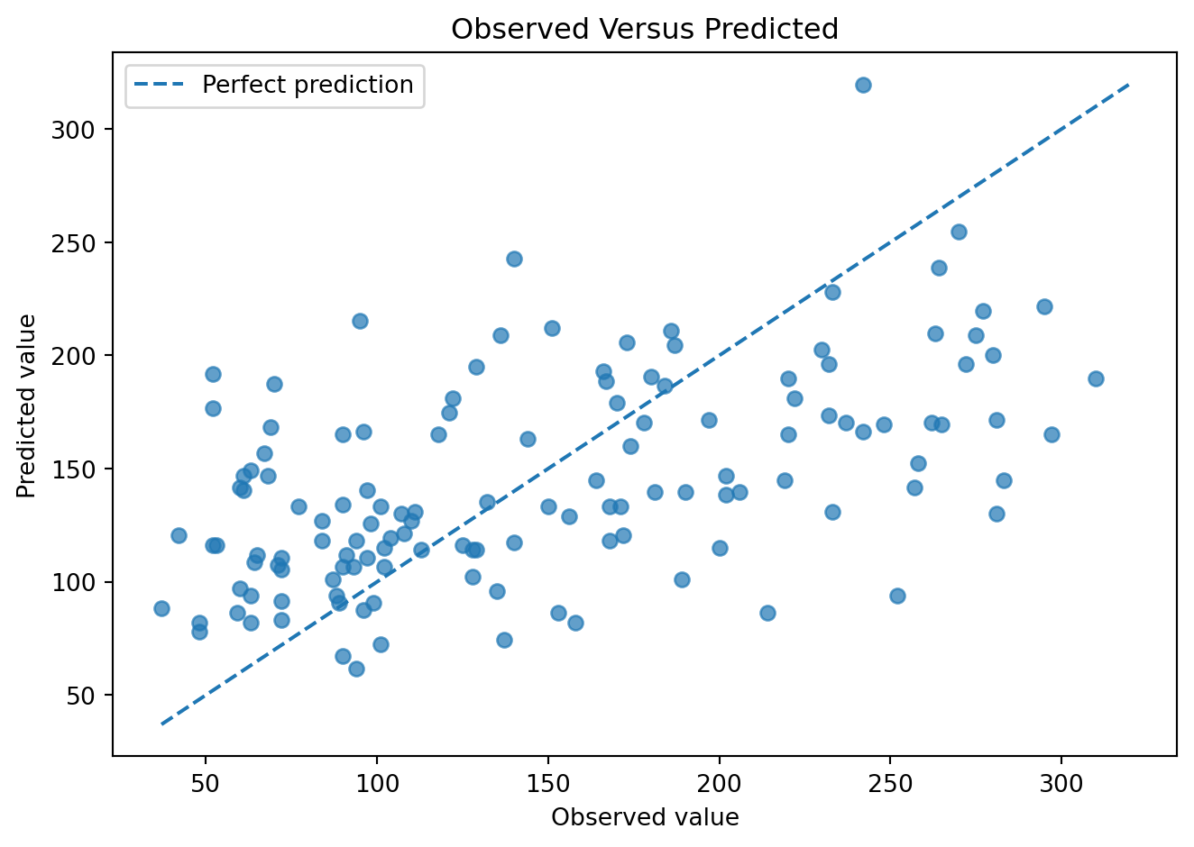
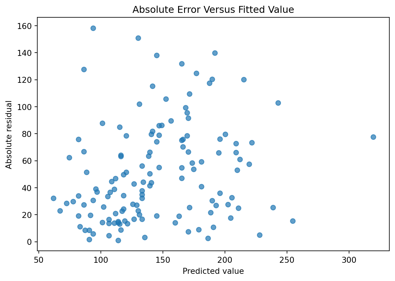
4.3. Residual Diagnostics

A scalar metric compresses many errors into one number. Residual plots reveal structure that the scalar hides.

Useful plots include:

• residual versus fitted value;
• residual versus each predictor;
• residual versus time;
• residual distribution;
• absolute residual versus fitted value;
• observed versus predicted;
• quantile–quantile plot;
• residuals by group or location.

Curvature

\[ \mathbb E[e\mid \hat y]\neq0 \]

suggests missing nonlinearity or interaction.

Fanning

\[ \operatorname{Var}(e\mid \hat y) \]

increases with fitted value, suggesting heteroskedasticity.

Temporal structure

\[ \operatorname{Corr}(e_t,e_{t-h})\neq0 \]

suggests omitted time dependence.

Group offsets

\[ \mathbb E[e\mid G=g] \]

differs across groups, suggesting systematic subgroup bias or missing contextual variables.

import numpy as np
import matplotlib.pyplot as plt

from sklearn.datasets import load_diabetes
from sklearn.linear_model import LinearRegression
from sklearn.model_selection import train_test_split
from sklearn.metrics import (
    mean_absolute_error,
    mean_squared_error,
    r2_score
)

data = load_diabetes()

bmi_index = list(data.feature_names).index("bmi")
X = data.data[:, [bmi_index]]
y = data.target

X_train, X_test, y_train, y_test = train_test_split(
    X,
    y,
    test_size=0.30,
    random_state=42
)

model = LinearRegression()
model.fit(X_train, y_train)

predicted = model.predict(X_test)
residuals = y_test - predicted

print("MAE:", mean_absolute_error(y_test, predicted))
print("RMSE:", mean_squared_error(
    y_test,
    predicted
) ** 0.5)
print("R²:", r2_score(y_test, predicted))

plt.figure(figsize=(7, 5))
plt.scatter(predicted, residuals, alpha=0.7)
plt.axhline(0, linestyle="--")
plt.title("Residuals Versus Fitted Values")
plt.xlabel("Predicted disease progression")
plt.ylabel("Residual")
plt.tight_layout()
plt.show()

plt.figure(figsize=(7, 5))
plt.scatter(y_test, predicted, alpha=0.7)
minimum = min(y_test.min(), predicted.min())
maximum = max(y_test.max(), predicted.max())
plt.plot(
    [minimum, maximum],
    [minimum, maximum],
    linestyle="--",
    label="Perfect prediction"
)
plt.title("Observed Versus Predicted")
plt.xlabel("Observed value")
plt.ylabel("Predicted value")
plt.legend()
plt.tight_layout()
plt.show()

plt.figure(figsize=(7, 5))
plt.scatter(
    predicted,
    np.abs(residuals),
    alpha=0.7
)
plt.title("Absolute Error Versus Fitted Value")
plt.xlabel("Predicted value")
plt.ylabel("Absolute residual")
plt.tight_layout()
plt.show()

MAE: 50.59307504375872
RMSE: 62.32926055201547
R²: 0.2803417492440603

4.4. Substantive Validity and Impossible Predictions

A regression model may minimize average error while producing impossible outputs:

• negative demand;
• probabilities above 1;
• negative recovery score;
• negative remaining lifetime;
• temperatures outside a physical operating range;
• revenue larger than the market itself.

Possible remedies include:

• transforming the target;
• using an appropriate response distribution;
• imposing constraints;
• modeling rates or proportions directly;
• adding monotonicity constraints;
• changing the model family.

A post-processing clip,

\[ \hat y_{\text{clipped}} = \min(b,\max(a,\hat y)), \]

may prevent impossible output but does not repair the underlying misspecification.

4.5. Prediction Intervals

A point prediction does not communicate uncertainty. A prediction interval seeks bounds \([L(x),U(x)]\) such that

\[ P \left( Y_{\mathrm{new}}\in[L(X_{\mathrm{new}}),U(X_{\mathrm{new}})] \right) \approx1-\alpha. \] Evaluation must include both:

Coverage

\[ \widehat{\operatorname{Coverage}} = \frac1N \sum_{i=1}^{N} I(y_i\in[L_i,U_i]). \]

Width

\[ \widehat W = \frac1N \sum_{i=1}^{N}(U_i-L_i). \]

Intervals that cover almost everything by being extremely wide are not useful. Coverage and sharpness must be considered together.

5. Classification Evaluation and Debugging

5.1. Confusion-Matrix Metrics

For binary classification:

\[ \operatorname{Precision} = \frac{TP}{TP+FP}, \] \[ \operatorname{Recall} = \frac{TP}{TP+FN}, \] \[ \operatorname{Specificity} = \frac{TN}{TN+FP}, \] \[ F_1 = 2 \frac{ \operatorname{Precision}\cdot\operatorname{Recall} }{ \operatorname{Precision}+\operatorname{Recall} }. \]

The \(F_\beta\) score weights recall relative to precision:

\[ F_\beta = (1+\beta^2) \frac{PR}{\beta^2P+R}. \] When \(\beta>1\), recall receives greater weight.

5.2. Accuracy Under Class Imbalance

Suppose 1% of transactions are fraudulent. A classifier predicting every transaction as legitimate has

\[ \operatorname{Accuracy}=0.99. \]

Yet \(\operatorname{Recall}=0\).

The correct baseline depends on the use case:

• majority-class classifier;
• existing business rules;
• random ranking;
• previous production model;
• manual review process;
• no-action policy.

A new model should beat the operational baseline, not merely a weak academic baseline.

5.3. ROC and Precision–Recall Curves

Given score \(s(x)\) and threshold \(t\):

\[ \begin{aligned} TPR(t) &= P(s(X)\geq t\mid Y=1),\\ FPR(t) &= P(s(X)\geq t\mid Y=0). \end{aligned} \]

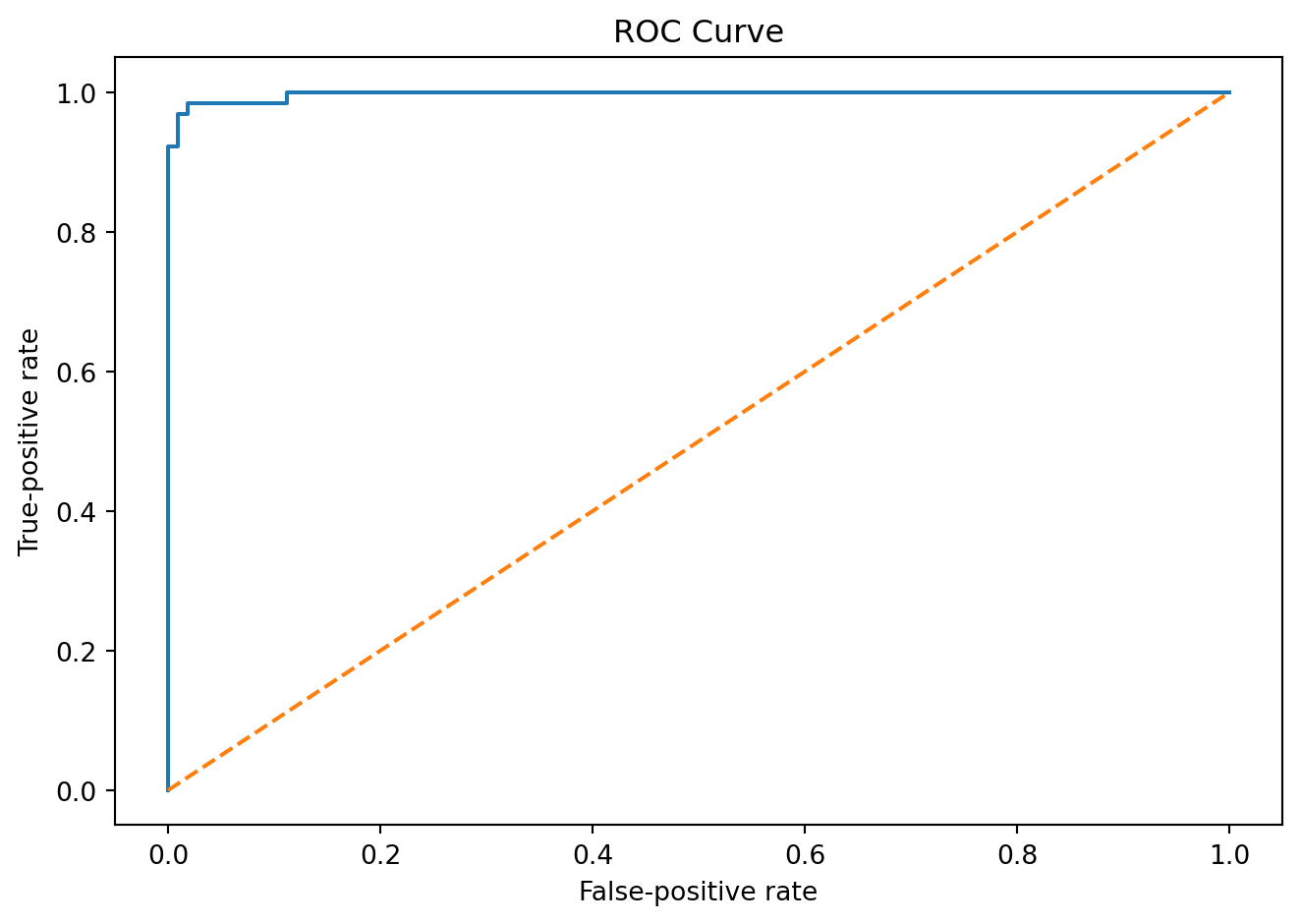
The ROC curve plots \(TPR(t)\) against \(FPR(t)\).

ROC-AUC has a ranking interpretation:

\[ AUC = P(s(X^+)>s(X^-)), \]

with a tie adjustment under discrete scores.

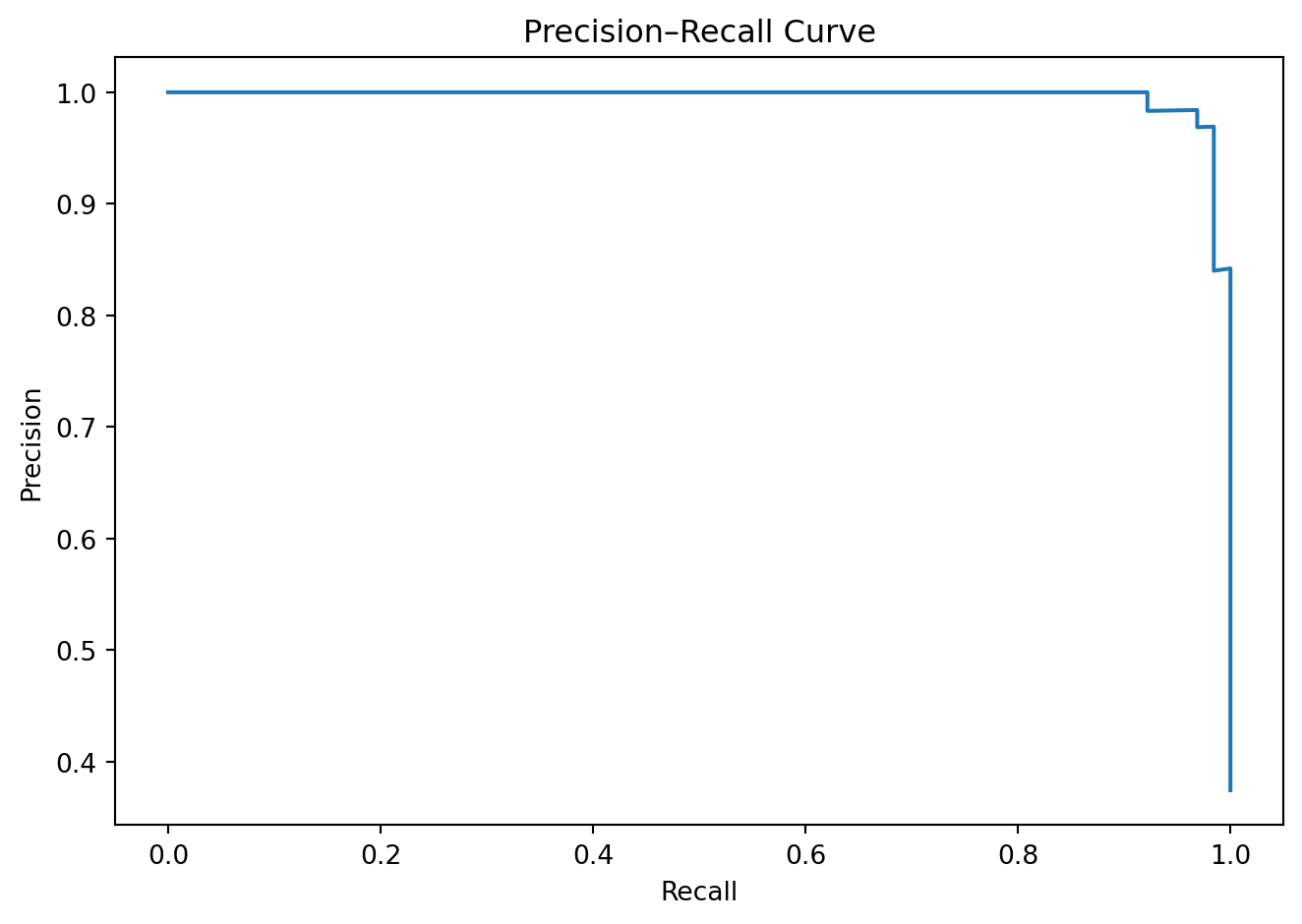
For rare positive classes, precision–recall curves are often more operationally informative because precision depends directly on prevalence:

\[ \operatorname{Precision} = \frac{ TPR\cdot P(Y=1) }{ TPR\cdot P(Y=1) + FPR\cdot P(Y=0) }. \]

Even a small false-positive rate can generate many false alerts when negatives are abundant.

import numpy as np
import pandas as pd
import matplotlib.pyplot as plt

from sklearn.datasets import load_breast_cancer
from sklearn.linear_model import LogisticRegression
from sklearn.metrics import (
    confusion_matrix,
    precision_recall_curve,
    roc_curve,
    roc_auc_score,
    average_precision_score
)
from sklearn.model_selection import train_test_split
from sklearn.pipeline import Pipeline
from sklearn.preprocessing import StandardScaler

data = load_breast_cancer()

X = data.data

# Convert malignant to positive class.
y = (data.target == 0).astype(int)

X_train, X_test, y_train, y_test = train_test_split(
    X,
    y,
    test_size=0.30,
    stratify=y,
    random_state=42
)

model = Pipeline([
    ("scaler", StandardScaler()),
    ("classifier", LogisticRegression(max_iter=3000))
])

model.fit(X_train, y_train)
probability = model.predict_proba(X_test)[:, 1]

print("ROC-AUC:", roc_auc_score(y_test, probability))
print(
    "PR-AUC:",
    average_precision_score(y_test, probability)
)

thresholds = [0.10, 0.25, 0.50, 0.75]
rows = []

for threshold in thresholds:
    predicted = (probability >= threshold).astype(int)
    tn, fp, fn, tp = confusion_matrix(
        y_test,
        predicted
    ).ravel()

    rows.append({
        "threshold": threshold,
        "TP": tp,
        "FP": fp,
        "FN": fn,
        "TN": tn,
        "precision": tp / (tp + fp) if tp + fp else 0,
        "recall": tp / (tp + fn) if tp + fn else 0
    })

print(pd.DataFrame(rows))

fpr, tpr, _ = roc_curve(y_test, probability)

plt.figure(figsize=(7, 5))
plt.plot(fpr, tpr)
plt.plot([0, 1], [0, 1], linestyle="--")
plt.title("ROC Curve")
plt.xlabel("False-positive rate")
plt.ylabel("True-positive rate")
plt.tight_layout()
plt.show()

precision, recall, _ = precision_recall_curve(
    y_test,
    probability
)

plt.figure(figsize=(7, 5))
plt.plot(recall, precision)
plt.title("Precision–Recall Curve")
plt.xlabel("Recall")
plt.ylabel("Precision")
plt.tight_layout()
plt.show()

ROC-AUC: 0.997517523364486
PR-AUC: 0.9962959459630412
   threshold  TP  FP  FN   TN  precision    recall
0       0.10  63   7   1  100   0.900000  0.984375
1       0.25  62   1   2  106   0.984127  0.968750
2       0.50  60   1   4  106   0.983607  0.937500
3       0.75  56   0   8  107   1.000000  0.875000

5.4. Capacity-Constrained Evaluation

Suppose a fraud-review team can inspect only 500 transactions per day. The relevant question is not performance at threshold 0.5. It is performance among the 500 highest-risk cases.

Useful metrics include:

Precision at k

\[ P@k = \frac{ \text{positive cases among top }k }{ k }. \]

Recall at k

\[ R@k = \frac{ \text{positive cases among top }k }{ \text{all positive cases} }. \]

Lift at k

\[ \operatorname{Lift}@k = \frac{P@k}{P(Y=1)}. \]

These metrics align evaluation with resource constraints.

5.5. Probability Calibration

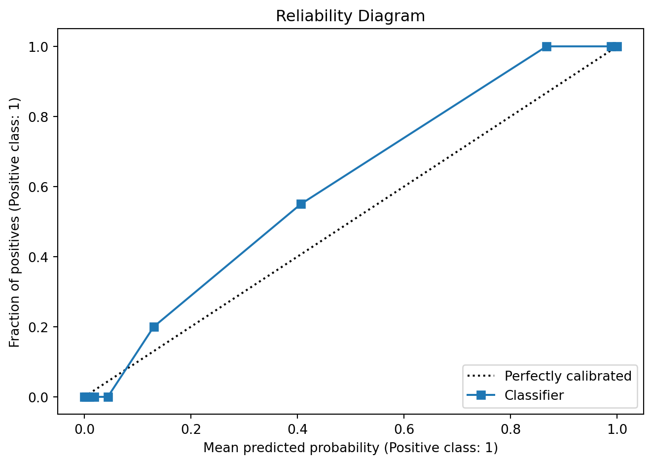
A classifier is calibrated when predicted probabilities correspond to observed frequencies.

For cases with \(\hat p(x)\approx0.8\), approximately 80% should be positive.

A model can rank cases well but be poorly calibrated. Guo et al. found that modern neural networks in their experiments could be miscalibrated and showed that temperature scaling was an effective post-hoc method in many evaluated settings³.

The Brier score is

\[ BS = \frac1N \sum_{i=1}^{N} (\hat p_i-y_i)^2. \]

It evaluates probabilistic predictions rather than hard classifications and traces to Brier’s work on verifying probability forecasts ⁴.

Log loss is

\[ LL = -\frac1N \sum_{i=1}^{N} \left[ y_i\log\hat p_i + (1-y_i)\log(1-\hat p_i) \right]. \]

Log loss strongly penalizes confident wrong predictions.

import matplotlib.pyplot as plt

from sklearn.calibration import CalibrationDisplay
from sklearn.datasets import load_breast_cancer
from sklearn.ensemble import RandomForestClassifier
from sklearn.model_selection import train_test_split
from sklearn.metrics import brier_score_loss

data = load_breast_cancer()
X = data.data
y = (data.target == 0).astype(int)

X_train, X_test, y_train, y_test = train_test_split(
    X,
    y,
    test_size=0.35,
    stratify=y,
    random_state=42
)

model = RandomForestClassifier(
    n_estimators=400,
    min_samples_leaf=2,
    random_state=42
)
model.fit(X_train, y_train)

probability = model.predict_proba(X_test)[:, 1]

print(
    "Brier score:",
    brier_score_loss(y_test, probability)
)

plt.figure(figsize=(7, 5))
CalibrationDisplay.from_predictions(
    y_test,
    probability,
    n_bins=10,
    strategy="quantile"
)
plt.title("Reliability Diagram")
plt.tight_layout()
plt.show()

Brier score: 0.03487893804487709

<Figure size 672x480 with 0 Axes>

6. Evaluating Unsupervised Models

6.1. Clustering

Clustering evaluation differs because no target is required during fitting.

Internal metrics include:

• within-cluster sum of squares;
• silhouette score;
• gap statistic;
• density connectivity;
• stability.

When external labels exist, one may compute:

• adjusted Rand index;
• normalized mutual information;
• purity.

However, an unsupervised cluster can be useful without matching an existing label. Conversely, a high agreement score does not guarantee operational value.

Important practical checks include:

• Does the solution persist across random seeds?
• Does it persist under resampling?
• Are clusters driven by a single scale-dominated variable?
• Are tiny clusters merely outliers?
• Can new observations be assigned?
• Do cluster profiles remain stable over time?
• Does acting on the segmentation produce value?

6.2. Dimensionality Reduction

For PCA and autoencoders, evaluation can include reconstruction error:

\[ R_M = \frac1N \sum_{i=1}^{N} \|x_i-\hat x_i^{(M)}\|^2. \]

Additional questions include:

• Are neighborhoods preserved?
• Are downstream models improved?
• Are rare cases destroyed?
• Are conclusions stable under scaling?
• Does the two-dimensional display represent enough variation?
• Are important structures hidden in later dimensions?

A visually appealing projection is not evidence that the embedding preserves every relevant relationship.

7. Numerical and Statistical Stability

7.1. Conditioning

A mathematical problem is ill-conditioned when small input perturbations produce large output changes.

For linear system \(Ax=b\), the condition number under the 2-norm is

\[ \kappa_2(A) = \|A\|_2\|A^{-1}\|_2 = \frac{\sigma_{\max}(A)} {\sigma_{\min}(A)}. \]

A large condition number indicates sensitivity.

In linear regression,

\[ \hat\beta = (X^\top X)^{-1}X^\top y. \]

Highly correlated columns make the smallest singular values of X small, increasing instability.

Symptoms include:

• large coefficient changes under small data perturbations;
• opposite coefficient signs across samples;
• huge standard errors;
• unstable selected variables;
• good prediction but unreliable attribution.

Possible responses include:

• removing redundant variables;
• ridge regularization;
• PCA or partial least squares;
• acquiring more varied data;
• reporting predictive rather than causal interpretations.

7.2. Backward Error

Forward error asks \(\|\hat x-x^*\|\), where \(x^*\) is the exact unknown solution.

Backward error asks:

What smallest perturbation to the original problem would make \(\hat x\) an exact solution?

For \(Ax=b\), the residual is

\[ r=b-A\hat x. \]

A small residual means \(\hat x\) solves a nearby equation well. However, in an ill-conditioned problem, a small residual does not guarantee a small forward error.

This distinction matters in optimization and numerical linear algebra. The algorithm may be numerically stable even when the statistical problem is intrinsically unstable.

7.3. Perturbation Testing

A practical sensitivity analysis repeatedly perturbs the data:

1. bootstrap observations;
2. add small measurement noise;
3. change preprocessing choices;
4. refit the model;
5. compare parameters and predictions.

For parameter vector \(\hat\theta^{(b)}\), inspect:

\[ \operatorname{Var}_b(\hat\theta^{(b)}). \]

For predictions at \(x\), inspect:

\[ \operatorname{Var}_b \left[ \hat f^{(b)}(x) \right]. \]

A model can have stable aggregate accuracy but unstable individual predictions. That instability matters when decisions are made at the individual level.

8. Dataset Shift and Production Failure

8.1. Training and Deployment Distributions

Offline evaluation usually assumes future observations resemble development observations.

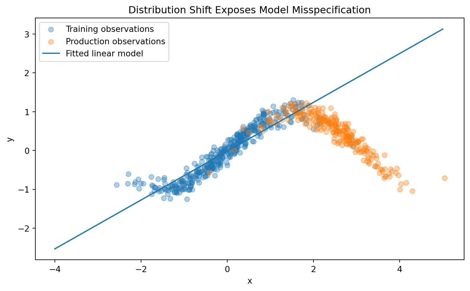
Let: \(P_{\mathrm{train}}(X,Y)\) be the development distribution and \(P_{\mathrm{prod}}(X,Y)\) the production distribution.

Dataset shift occurs when

\[ P_{\mathrm{train}}(X,Y) \neq P_{\mathrm{prod}}(X,Y). \]

Common forms include:

Covariate shift

\[ P_{\mathrm{train}}(X) \neq P_{\mathrm{prod}}(X), \]

but

\[ P_{\mathrm{train}}(Y\mid X) = P_{\mathrm{prod}}(Y\mid X). \]

Label shift

\[ P_{\mathrm{train}}(Y) \neq P_{\mathrm{prod}}(Y), \]

with approximately stable \(P(X\mid Y)\).

Concept shift

\[ P_{\mathrm{train}}(Y\mid X) \neq P_{\mathrm{prod}}(Y\mid X). \]

Dataset shift is a broad family of problems in which training and deployment distributions differ; covariate shift is only one special case.

8.2. Importance Weighting

Under covariate shift, production risk is

\[ R_{\mathrm{prod}}(f) = \mathbb E_{\mathrm{prod}} [L(Y,f(X))]. \]

Assuming stable conditional outcome distribution,

\[ P_{\mathrm{prod}}(Y\mid X) = P_{\mathrm{train}}(Y\mid X), \]

we can write

\[ R_{\mathrm{prod}}(f) = \mathbb E_{\mathrm{train}} \left[ w(X)L(Y,f(X)) \right], \] where \(w(x) = \frac{ p_{\mathrm{prod}}(x) }{ p_{\mathrm{train}}(x) }.\)

This suggests a weighted empirical objective:

\[ \widehat R_w(f) = \frac1N \sum_{i=1}^{N} w(x_i)L(y_i,f(x_i)). \]

In practice, density-ratio estimation can be difficult, and large weights increase variance. Reweighting is not a universal repair for arbitrary production failure.

8.3. Detecting Input Drift

For numerical feature \(X_j\), compare training and recent production distributions using:

• mean and variance;
• quantiles;
• missingness rate;
• range violations;
• population stability index;
• Kolmogorov–Smirnov distance;
• Wasserstein distance;
• learned two-sample classifiers.

A simple standardized mean difference is

\[ SMD_j = \frac{ \bar x_{j,\mathrm{prod}} - \bar x_{j,\mathrm{train}} }{ s_{j,\mathrm{pooled}} }. \]

For categorical features, compare category frequencies and unseen-category rates.

Drift does not automatically imply performance loss. A feature may drift without affecting predictions. Conversely, performance may degrade without obvious marginal drift if relationships among variables change.

import numpy as np
import matplotlib.pyplot as plt

from sklearn.linear_model import LinearRegression
from sklearn.metrics import mean_squared_error

rng = np.random.default_rng(42)

# Training inputs concentrated near zero.
x_train = rng.normal(0, 1.0, size=400)
y_train = (
    np.sin(x_train)
    + 0.15 * rng.normal(size=len(x_train))
)

# Production inputs shift toward a region poorly represented in training.
x_production = rng.normal(2.5, 0.8, size=250)
y_production = (
    np.sin(x_production)
    + 0.15 * rng.normal(size=len(x_production))
)

model = LinearRegression()
model.fit(x_train.reshape(-1, 1), y_train)

train_prediction = model.predict(
    x_train.reshape(-1, 1)
)
production_prediction = model.predict(
    x_production.reshape(-1, 1)
)

print(
    "Training RMSE:",
    mean_squared_error(
        y_train,
        train_prediction
    ) ** 0.5
)

print(
    "Production RMSE:",
    mean_squared_error(
        y_production,
        production_prediction
    ) ** 0.5
)

grid = np.linspace(-4, 5, 400)
grid_prediction = model.predict(grid.reshape(-1, 1))

plt.figure(figsize=(8, 5))
plt.scatter(
    x_train,
    y_train,
    alpha=0.35,
    label="Training observations"
)
plt.scatter(
    x_production,
    y_production,
    alpha=0.35,
    label="Production observations"
)
plt.plot(
    grid,
    grid_prediction,
    label="Fitted linear model"
)
plt.title("Distribution Shift Exposes Model Misspecification")
plt.xlabel("x")
plt.ylabel("y")
plt.legend()
plt.tight_layout()
plt.show()

Training RMSE: 0.26750159054323086
Production RMSE: 1.4247840786736916

9. Subgroup Performance and Fairness

9.1. Aggregate Metrics Can Hide Failure

Suppose two groups have sizes \(n_A\) and \(n_B\). Aggregate error is

\[ R = \frac{ n_AR_A+n_BR_B }{ n_A+n_B }. \]

If \(n_A\gg n_B\), poor performance in group \(B\) may barely affect the overall metric.

Evaluation should therefore examine:

• performance by demographic group;
• performance by location;
• performance by device type;
• performance by time;
• performance by severity;
• performance by data-quality level;
• performance for rare and high-cost cases.

These slices should be planned before inspecting results when possible, because searching many slices can create false discoveries.

9.2. Relevant Group Metrics

For classification, possible comparisons include:

True-positive rate

\[ TPR_g = P(\hat Y=1\mid Y=1,G=g). \]

False-positive rate

\[ FPR_g = P(\hat Y=1\mid Y=0,G=g). \]

Positive predictive value

\[ PPV_g = P(Y=1\mid\hat Y=1,G=g). \]

Calibration by group

\[ P(Y=1\mid\hat p=p,G=g)\approx p. \]

These criteria cannot always be satisfied simultaneously when group base rates differ. Therefore, fairness evaluation requires explicit decisions about the relevant harms and institutional context.

---

The purpose of modeling is not to produce an elegant fitted function. It is to support reliable understanding and effective action.

Evaluation begins by separating training, model selection, and final assessment. Cross-validation, bootstrap methods, temporal splits, spatial splits, and grouped splits are not interchangeable conventions. They represent different claims about how the model will generalize.

Leakage is among the most dangerous evaluation failures because it can produce strong apparent performance without genuine predictive information. Every operation that learns from data—including scaling, feature selection, imputation, PCA, threshold selection, and hyperparameter tuning—must be contained within the appropriate training partition.

Metrics must match the decision. RMSE and MAE correspond to different error priorities. Accuracy can be meaningless under imbalance. ROC-AUC evaluates ranking but not operational thresholds. Precision, recall, calibration, top-k performance, and expected cost answer different questions. No single metric is universally sufficient.

Debugging requires more than comparing scalar scores. Residual plots reveal nonlinear misspecification, heteroskedasticity, temporal dependence, and subgroup failure. Sensitivity analysis reveals unstable parameters and predictions. Calibration diagnostics reveal whether reported probabilities are trustworthy. Learning curves indicate whether the limiting factor is bias, variance, or insufficient data.

Production evaluation expands the object of analysis from the model to the entire system. Feature pipelines, database joins, software versions, thresholds, human review, latency, and feedback loops can determine whether an apparently strong model succeeds or fails. A production model must therefore be tested and monitored as a data-dependent software system, not merely as a mathematical function.

Stakeholders rarely need every derivation underlying the model. They need clear answers:

• Does it improve the current process?
• What does it cost?
• Which errors remain?
• Who is harmed when it fails?
• How many cases can be processed?
• What evidence supports deployment?
• How will failure be detected?
• How quickly can the system be rolled back?

The strongest final model is not necessarily the most complicated or the most accurate under one benchmark. It is the model whose evidence, decision value, operational behavior, and limitations are understood well enough that the organization can use it responsibly.

Previous chapter: Data Modeling - Clustering

Footnotes

1. Sculley, D., Gary Holt, Daniel Golovin, et al. “Hidden Technical Debt in Machine Learning Systems.” Advances in Neural Information Processing Systems 28 (2015). https://proceedings.neurips.cc/paper_files/paper/2015/hash/86df7dcfd896fcaf2674f757a2463eba-Abstract.html.

2. Efron, Bradley, and Robert Tibshirani. “Improvements on Cross-Validation: The 632+ Bootstrap Method.” Journal of the American Statistical Association 92, no. 438 (1997): 548–60. https://doi.org/10.1080/01621459.1997.10474007.

3. Guo, Chuan, Geoff Pleiss, Yu Sun, and Kilian Q. Weinberger. “On Calibration of Modern Neural Networks.” Proceedings of the 34th International Conference on Machine Learning, July 17, 2017, 1321–30. https://proceedings.mlr.press/v70/guo17a.html.

4. Brier, Glenn W. VERIFICATION OF FORECASTS EXPRESSED IN TERMS OF PROBABILITY. Monthly Weather Review. January 1, 1950. https://journals.ametsoc.org/view/journals/mwre/78/1/1520-0493_1950_078_0001_vofeit_2_0_co_2.xml.