Data Modeling - KNN

While regression models approximate an unknown relationship through a mathematical function and tree-based models approximate the response by recursively partitioning the feature space into regions, K-Nearest Neighbors, usually abbreviated as KNN or \(\mathbf k\)-NN, predicts by comparing a new observation to the most similar observations already seen. KNN is a non-parametric, instance-based, and memory-based learning method.

This chapter studies KNN as a mathematical model of local constancy. The basic assumption is:

Points close to each other in feature space tend to have similar responses.

For classification, this means nearby points tend to share the same class label. For regression, nearby points tend to have similar numerical target values. KNN is therefore sometimes used in unsupervised learning tasks.

KNN is often called a lazy learner because it performs almost no explicit model fitting during training. The training phase stores the data. The main computational work happens during prediction, when the algorithm searches for the nearest training points to a query point.

1. Formal Setup

Let the training data be

\[ \mathcal D_n = \{(x_i, y_i)\}_{i=1}^n \]

where \(x_i\in \mathbb R^p\) is a feature vector with \(p\) variables.

For classification, \(y_i\in \{1, 2, \dots, K\}\). For regression, \(y_i\in \mathbb R\).

Let

\[ d: \mathcal X \times \mathcal X \to [0, \infty) \]

be a distance function. For a query point \(x\), KNN identifies the \(k\) training points closest to \(x\).

NoteDefinition: K-Nearest Neighbor Set

Given a query point \(x\), a distance function \(d\), and an integer \(k\geq 1\), the \(k\)-nearest neighbor set of \(x\) is

\[ N_k(x) = \{i_1, i_2, \dots, i_k\}, \]

where

\[ d(x, x_{i_1}) \leq d(x, x_{i_2}) \leq \dots \leq d(x, x_{i_k}) \]

and \(i_1, \dots, i_k\) are the indices of the \(k\) closest training observations to \(x\).

If ties occur, they are usually broken arbitrarily or according to an implementation-specific rule. The KNN prediction depends entirely on \(N_k(x)\).

2. Distance, Geometry, and Similarity

KNN does not learn coefficients, tree splits, or any weights. Instead, the distance function determines the geometry of the model.

A distance function decides which points count as similar. Therefore, choosing a distance metric equivalent to choosing the model’s notion of relevance.

TipExample

In a medical dataset, two patients may be close if they have similar age, blood pressure, cholesterol, and heart rate. In a text dataset, two documents may be close if they use similar vocabulary. In a recommender system, two users may be close if they rate the same movies similarly.

Thus, KNN depends on the question:

What does similarity mean in this problem?

2.1. Metric Spaces

NoteDefinition: Metric

A function \(d:\mathcal X \times \mathcal X \to [0, \infty)\) is a metric if for all \(x, y, z \in \mathcal X\), it satisfies:

1. Non-negativity: \(d(x, y) \geq 0\).
2. Identify of indiscernibles: \(d(x, y)=0 \Leftrightarrow x=y\).
3. Symmetry: \(d(x, y) = d(y,x)\).
4. Triangle inequality: \(d(x, z) \leq d(x, y) + d(y, z)\).

Not every similarity score is a metric. Cosine similarity, for example, is usually a similarity measure rather than a metric, although related angular distances can be constructed.

2.2. Euclidean Distance

The most common distance for numerical data is Euclidean distance:

\[ d_2(x, z) = \sqrt{\sum_{j=1}^p (x_j-z_j)^2}. \]

This is the ordinary straight-line distance in \(p\)-dimensional space.

Euclidean distance is appropriate when:

• feature are continuous,
• features are on comparable scales,
• straight-line geometric proximity is meaningful,
• correlations among features are not severe.

The squared Euclidean distance is

\[ d^2_2(x, z) = \sum_{j=1}^p (x_j- z_j)^2 \]

Because the square root is monotone increasing, ranking neighbors by Euclidean distance is equivalent to ranking them by squared Euclidean distance.

TipExample

If \(x=(2,3)\) and \(z=(5,7)\), then

\[ d_2(x, z) = \sqrt{(2-5)^2 + (3-7)^2} = \sqrt{9+16}= 5 \]

2.3. Manhattan Distance

The Manhattan distance, or \(L_1\) distance, is

\[ d_1(x, z) = \sum_{j=1}^p |x_j-z_j|. \]

It measures the total axis-aligned movement required to travel from \(x\) to \(z\).

TipExample

If \(x=(2,3)\) and \(z=(5,7)\), then

\[ d_1(x, z) = |2-5| + |3-7| = 3 + 4 = 7 \]

Manhattan distance is often useful when movement or differences is naturally axis-aligned, such as city-block distance, sparse high-dimensional data, or feature spaces where additive deviations are more meaningful than squared deviations.

2.4. Minkowski Distance

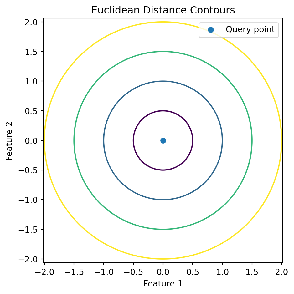
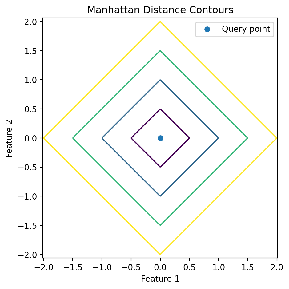
Euclidean and Manhattan distances are special cases of the Minkowski distance:

\[ d_q(x, z) = \left(\sum_{j=1}^p|x_j-z_j|^q\right)^{1/q} \]

where \(q\geq 1\).

Special cases: \(q=1\implies d_q=d_1\) is Manhattan distance, and \(q=2\implies d_q=d_2\) is Euclidean distance. As \(q\) changes, the geometry of neighborhoods changes.

2.5. Cosine Similarity

For text, social media, recommendation systems, and other sparse vector spaces, magnitude may be less important than direction. In such cases, cosine similarity is often used:

\[ \mathrm{cosine}(x, z) = \frac{x^\top z}{||x||_2 ||z||_2} \]

The corresponding cosine distance is commonly written as

\[ d_{\cos}(x, z)= 1- \frac{x^\top z}{||x||_2 ||z||_2} \]

Cosine similarity measures the angle between two vectors. If two documents use similar relative word patterns, they can have high cosine similarity even if one document is much longer than the other.

TipExample

Suppose \(x=(1,1,0)\) and \(z=(10,10,0)\). Then \(z=10x\), so they point in exactly the same direction. Their cosine similarity is

\[ \frac{x^\top z}{||x||_2||z||_2}=\frac{1\times 10 + 1\times 10}{\sqrt 2 \times 10\sqrt {2}}=1 \]

Thus, cosine similarity treats them as maximally similar in direction, even though their Euclidean distance is large.

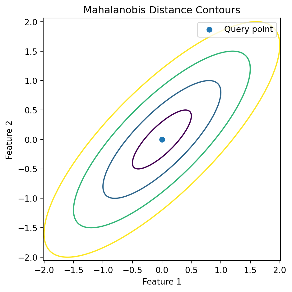
2.6. Mahalanobis Distance

Euclidean distance treats all coordinates as independent and equally scaled. This can be inappropriate when features are correlated.

The Mahalanobis distance is

\[ d_M (x,z) = \sqrt{(x-z)^\top \Sigma^{-1}(x-z)} \]

where \(\sigma\) is the covariance matrix of the features.

If \(\sigma=I\), then \(d_M(x, z) = d_2(x,z)\). If features are correlated, Mahalanobis distance rescales and rotates the geometry according to the covariance structure.

Caution

Mahalanobis distance is a multivariate generalization of the \(z\)-score. A point is far away if it is unusual relative to the covariance pattern of the data.

This is useful when two features move together. For example, height and weight are correlated. A person who is both taller and heavier may not be unusual, but a person with an unusual combination of height and weight may be far in Mahalanobis distance.

import numpy as np
import matplotlib.pyplot as plt

x = np.linspace(-2, 2, 400)
y = np.linspace(-2, 2, 400)
X, Y = np.meshgrid(x, y)

euclidean = np.sqrt(X**2 + Y**2)
manhattan = np.abs(X) + np.abs(Y)

# Mahalanobis with correlated covariance
Sigma = np.array([[1.0, 0.8],
                  [0.8, 1.0]])
Sigma_inv = np.linalg.inv(Sigma)

points = np.stack([X.ravel(), Y.ravel()], axis=1)
mahal = np.sqrt(np.sum(points @ Sigma_inv * points, axis=1)).reshape(X.shape)

for Z, title in [
    (euclidean, "Euclidean Distance Contours"),
    (manhattan, "Manhattan Distance Contours"),
    (mahal, "Mahalanobis Distance Contours")
]:
    plt.figure(figsize=(5, 5))
    plt.contour(X, Y, Z, levels=[0.5, 1.0, 1.5, 2.0])
    plt.scatter([0], [0], label="Query point")
    plt.title(title)
    plt.xlabel("Feature 1")
    plt.ylabel("Feature 2")
    plt.axis("equal")
    plt.legend()
    plt.tight_layout()
    plt.show()

(a) Comparing Distance Geometries

(b)

(c)

Figure 1

3. KNN Classification

3.1. KNN Classification Rule

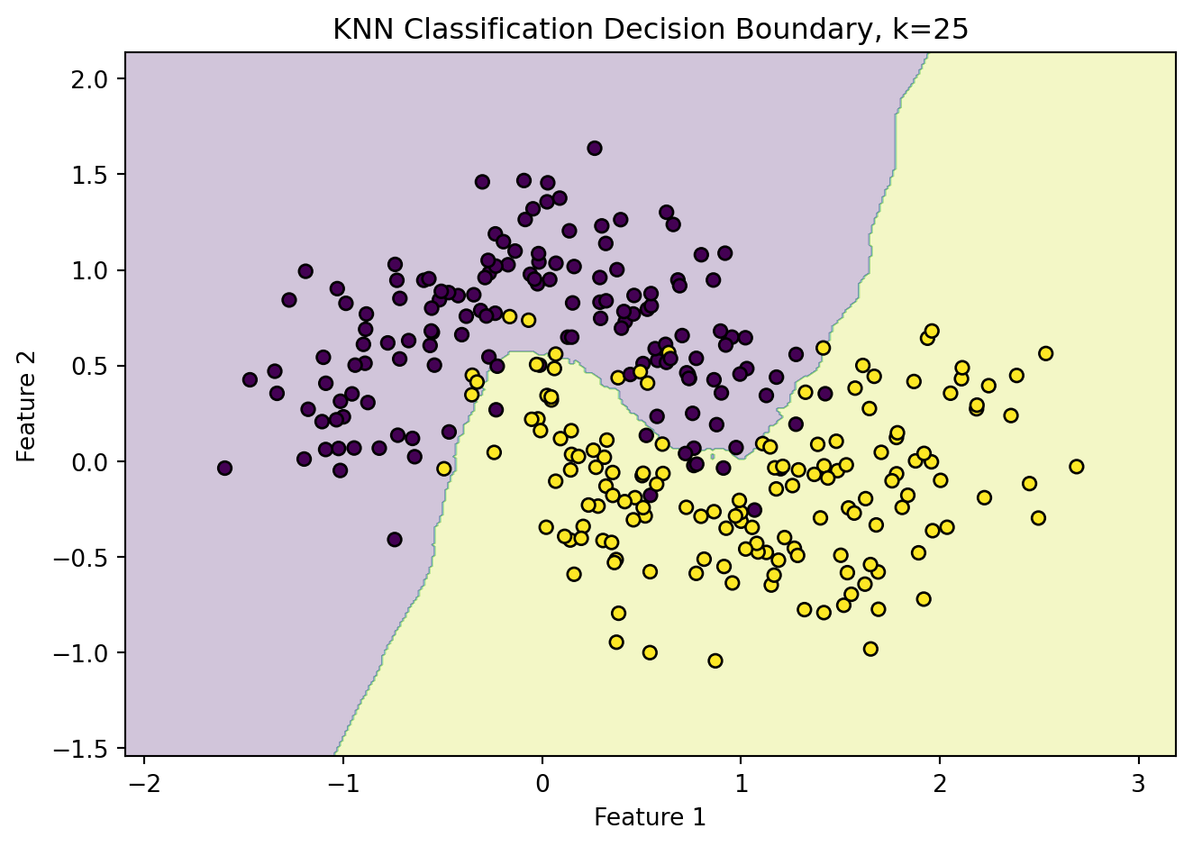
For classification, the KNN classifier predicts the most common class among the \(k\) nearest neighbors. Let \(Y\in \{1, \dots, K\}\).

For a query point \(x\), we define the estimated class probability

\[ \hat p_k(c|x) =\frac{1}{k}\sum_{i\in N_k(x)}\mathbf{I}\{y_i=c\} \]

where \(c\in \{1,\dots, K\}\). The KNN classification rule is

\[ \hat y(x) = \arg\max_{c\in \{1, \dots, K\}}\hat p_k(c|x) \]

Equivalently,

\[ \hat y(x) = \arg\max_c \sum_{i\in N_k(x)}\mathbf{I}\{y_i=c\}. \] This is majority voting.

3.2. Special Case: 1-Nearest Neighbor

When \(k=1\), the prediction is simply \(\hat y(x) = y_{i^*}\), where

\[ i^* = \arg\min_i d(x, x_i)/ \]

Thus, the query point receives the label of its single nearest training observation.

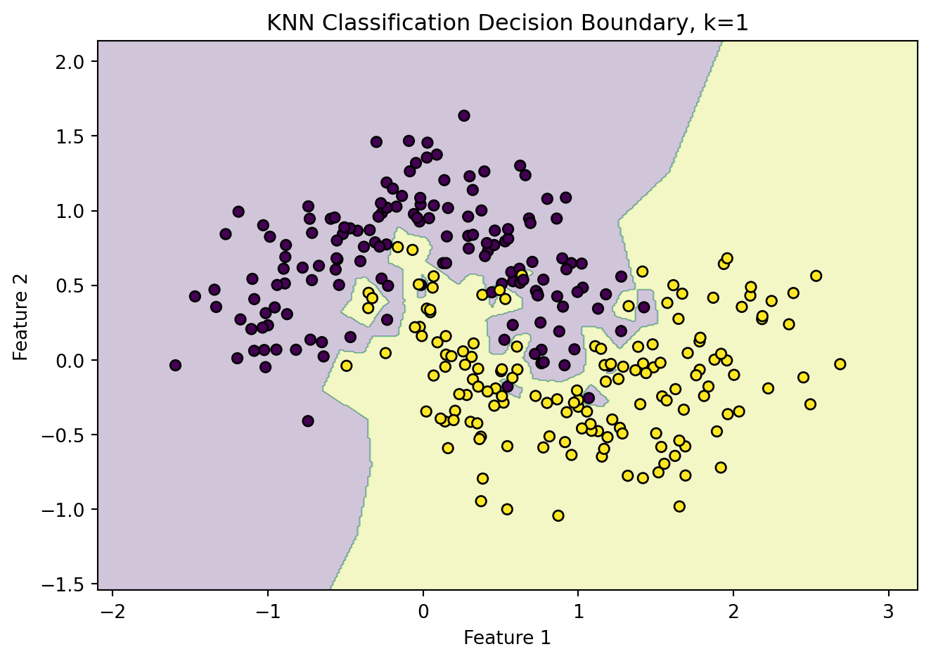
The 1-NN classifier produces highly flexible decision boundaries. In two dimensions, the decision regions correspond to a Voronoi tessellation of the training data. Each training point owns the region of the feature space closer to it than to any other training point.

Voronoi diagram

3.3. Weighted KNN Classification

Ordinary KNN gives equal weight to all \(k\) neighbors. But a neighbor very close to the query point may be more relevant than a neighbor near the edge of the neighborhood.

Weighted KNN assigns weights

\[ w_i(x) = K(d(x, x_i)) \]

where \(K(\cdot)\) is a decreasing function of distance.

A common inverse-distance weight is

\[ w_i(x) = \frac{1}{d(x, x_i)+\epsilon}, \]

where \(\epsilon>0\) prevents division by zero.

A Gaussian kernel weight is

\[ w_i(x) = \exp\left(-\frac{d(x, x_i)^2}{2h^2}\right), \]

where \(h>0\) is a bandwidth parameter.

The weighted class probability estimate is

\[ \hat {p}(c|x) = \frac{\sum_{i\in N_k(x)}w_i(x)\mathbf{I}\{y_i=c\}}{\sum_{i\in N_k(x)} w_i(x)} \]

The weighted KNN prediction is

\[ \hat y(x) = \arg \max_c \hat p(c|x) \]

import numpy as np
import matplotlib.pyplot as plt
from sklearn.datasets import make_moons
from sklearn.neighbors import KNeighborsClassifier

X, y = make_moons(n_samples=300, noise=0.25, random_state=42)

x_min, x_max = X[:, 0].min() - 0.5, X[:, 0].max() + 0.5
y_min, y_max = X[:, 1].min() - 0.5, X[:, 1].max() + 0.5

xx, yy = np.meshgrid(
    np.linspace(x_min, x_max, 400),
    np.linspace(y_min, y_max, 400)
)

grid = np.c_[xx.ravel(), yy.ravel()]

for k in [1, 5, 25, 75]:
    clf = KNeighborsClassifier(n_neighbors=k)
    clf.fit(X, y)

    Z = clf.predict(grid).reshape(xx.shape)

    plt.figure(figsize=(7, 5))
    plt.contourf(xx, yy, Z, alpha=0.25)
    plt.scatter(X[:, 0], X[:, 1], c=y, edgecolor="k", s=30)
    plt.title(f"KNN Classification Decision Boundary, k={k}")
    plt.xlabel("Feature 1")
    plt.ylabel("Feature 2")
    plt.tight_layout()
    plt.show()

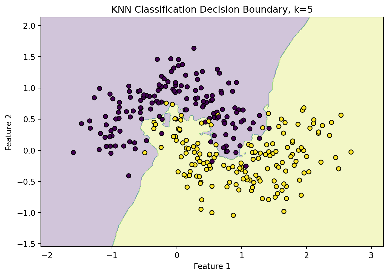
(a) KNN Classification Decision Boundaries

(b)

(c)

(d)

Figure 2

4. KNN Regression

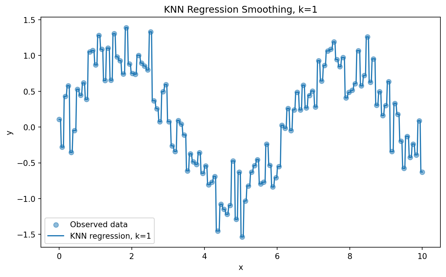
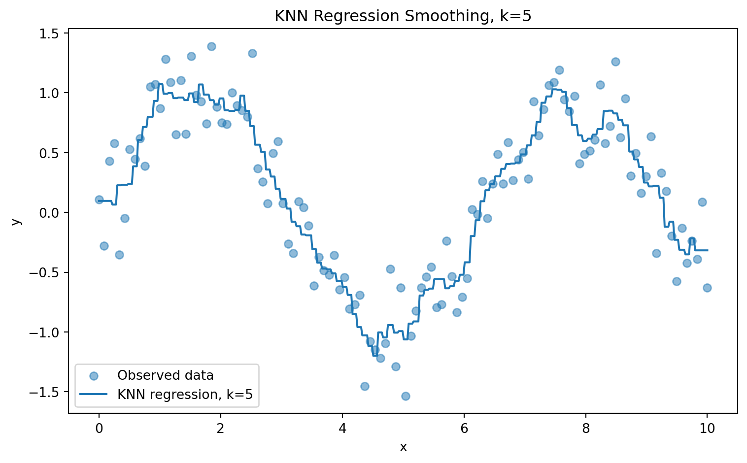
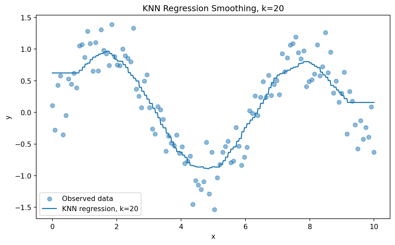
For regression, \(Y\in \mathbb R\). The KNN regression estimate is the average response of the \(k\) nearest neighbors:

\[ \hat f(x) = \frac{1}{k}\sum_{i\in N_k(x)}y_i \]

This is a local average estimator.

Weighted KNN regression is

\[ \hat f(x) = \frac{\sum_{i\in N_k(x)}w_i(x)y_i}{\sum_{i\in N_k(x)}w_i(x)} \]

If the weights are Gaussian,

\[ w_i(x) = \exp\left(-\frac{d(x,x_i)^2}{2h^2}\right) \]

then closer observations contribute more strongly to the prediction. This places KNN regression near the family of local smoothing methods.

TipTheorem: KNN Regression as a Local Constant Estimator

For a fixed neighborhood \(N_k(x)\), the KNN regression prediction

\[ \hat f_k(x) = \frac{1}{k}\sum_{i\in N_k(x)}y_i \]

is the constant \(c\) that minimizes the local squared-error objective

\[ J(c) = \sum_{i\in N_k(x)}(y_i-c)^2 \]

The proof is similar to the proof.

import numpy as np
import matplotlib.pyplot as plt
from sklearn.neighbors import KNeighborsRegressor

rng = np.random.default_rng(42)

X = np.linspace(0, 10, 120).reshape(-1, 1)
y = np.sin(X).ravel() + 0.35 * rng.normal(size=X.shape[0])

X_grid = np.linspace(0, 10, 500).reshape(-1, 1)

for k in [1, 5, 20, 60]:
    model = KNeighborsRegressor(n_neighbors=k)
    model.fit(X, y)

    y_pred = model.predict(X_grid)

    plt.figure(figsize=(8, 5))
    plt.scatter(X, y, alpha=0.5, label="Observed data")
    plt.plot(X_grid, y_pred, label=f"KNN regression, k={k}")
    plt.title(f"KNN Regression Smoothing, k={k}")
    plt.xlabel("x")
    plt.ylabel("y")
    plt.legend()
    plt.tight_layout()
    plt.show()

(a) KNN Regression Smoothing

(b)

(c)

(d)

Figure 3

5. Bias, Variance, and the Choice of \(k\).

5.1. Model Complexity in KNN

In KNN, the main complexity parameter is \(k\). Unlike tree depth or polynomial degree, KNN complexity moves in the opposite direction:

• small \(k\) means high complexity,
• large \(k\) means low complexity.

When \(k=1\), each prediction depends on a single point. This gives a very flexible model. When \(k=n\), every prediction uses the entire training set. For regression, \(\hat f_n(x) = \overline y\), which is just the global mean and ignores \(x\). For classification, \(k=n\) predicts the majority class everywhere.

5.2. Bias-Variance Interpretation

Let the true regression function be

\[ f(x) = \mathbb E[Y|X=x] \]

KNN regression estimates \(f(x)\) by averaging nearby response. The behavior depends on the neighborhood radius.

For small \(k\), the neighborhood is small. The estimate is local, so bias is low. But it uses few observations, so variance is high.

For large \(k\), the neighborhood is large. The estimate uses many observations, so variance is lower. But the neighborhood may include points where \(f(x)\) is different, so bias is higher.

5.3. Choosing \(k\) by Cross validation

The usual practical method for choosing \(k\) is cross-validation. For candidate values \(k\in \mathcal K\), fit KNN models and estimate validation error. Choose \(\hat k =\arg\min_{k\in\mathcal K}CV(k)\).

For regression, a common cross-validation score is

\[ CV(k) = \frac{1}{V} \sum_{v=1}^V\frac{1}{|I_v|}\sum_{i\in I_v} (y_i-\hat f_k^{(-v)}(x_i))^2 \]

Here:

• \(V\) is the number of folds,
• \(I_v\) is the validation fold,
• \(\hat f_k^{-(v)}\) is the model trained without fold \(v\).

For classification, one may use validation error:

\[ CV(k) = \frac{1}{V} \sum_{v=1}^V \frac{1}{|I_v|}\sum_{i\in I_v}\mathbf{I}\{y_i\neq \hat y_k^{(-v)}(x_i)\}. \]

import numpy as np
import matplotlib.pyplot as plt
from sklearn.datasets import make_moons
from sklearn.neighbors import KNeighborsClassifier
from sklearn.model_selection import cross_val_score

X, y = make_moons(n_samples=400, noise=0.3, random_state=42)

k_values = list(range(1, 61))
cv_errors = []

for k in k_values:
    clf = KNeighborsClassifier(n_neighbors=k)
    scores = cross_val_score(clf, X, y, cv=5, scoring="accuracy")
    cv_errors.append(1 - scores.mean())

best_k = k_values[int(np.argmin(cv_errors))]

plt.figure(figsize=(8, 5))
plt.plot(k_values, cv_errors, marker="o")
plt.axvline(best_k, linestyle="--", label=f"Best k = {best_k}")
plt.title("Choosing k by Cross-Validation")
plt.xlabel("Number of neighbors k")
plt.ylabel("Cross-validation error")
plt.legend()
plt.tight_layout()
plt.show()

Figure 4: Cross Validation Curve for k

6. Statistical Theory

6.1. The Cover-Hart Theorem

KNN has an important classical theoretical guarantee. Let \(R^*\) be the Bayes error rate, meaning the lowest possible classification error achievable by any classifier under the true data-generating distribution. Let \(R_{1NN}\) be the asymptotic error rate of the 1-nearest-neighbor classifier as the training sample size tends to infinity.

TipTheorem: Cover-Hart Bound

Under suitable regularity conditions,

\[ R^* \leq R_{1NN} \leq 2R^*(1-R^*) \]

Since

\[ 1-R^* \leq 1 \]

we have

\[ R_{1NN}\leq 2R^* \]

Thus, asymptotically, the 1-nearest-neighbor classifier has error no more than twice the Bayes error¹.

This theorem is important because 1-NN is extremely simple. It does not estimate a parametric model. It does not assume linearity. It merely copies the label of the closest training point. Yet, under increasing sample size, its error is theoretically controlled by the Bayes error.

However, the theorem does not say that 1-NN is always optimal. It says that its asymptotic error is bounded. In finite samples, especially high-dimensional or noisy data, 1-NN may perform poorly due to high variance.

6.2. Consistency of KNN

A classifier is consistent if its error rate approaches the Bayes error rate as

\[ n\to\infty \]

The 1-NN classifier is not generally Bayes consistent because its asymptotic error may remain above \(R^*\). But \(k\)-NN can be consistent if \(k\) grows with \(n\) at the right rate.

A standard condition is

\[ k\to \infty, \quad \frac{k}{n}\to 0 \]

as \(n\to\infty\).

The first condition ensures that the local estimate averages over enough points to reduce variance. The second condition ensures that the neighborhood remains local, so bias goes to zero.

7. The Curse of Dimensionality

KNN relies on the idea that nearby points are informative. But in high-dimensional spaces, points become sparse. The nearest neighbor may no longer be close in a meaningful sense.

This is an instance of the curse of dimensionality discussed previously. Here, the problem is geometric: as \(p\) increase, the volume of the feature space grows so quickly that the data become locally sparse.

For KNN, this means \(N_k(x)\) may contain points that are not truly similar to \(x\). The local constancy assumption fails.

7.1. Volume Argument

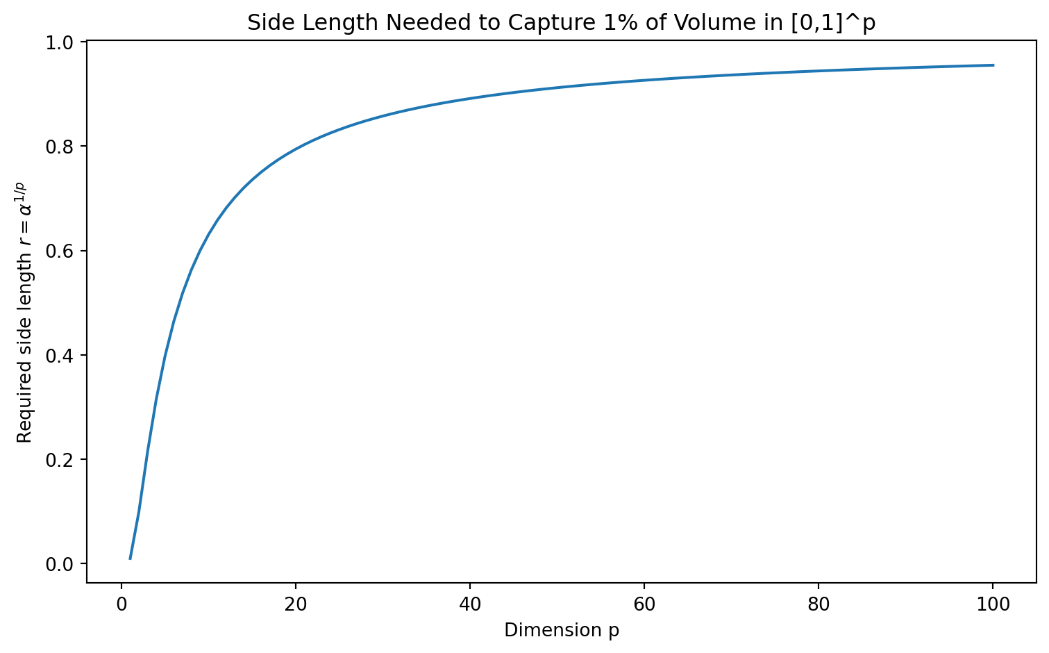
Consider the unit hypercube \([0,1]^p\). Suppose data are uniformly distributed in this cube. A smaller hypercube with side length \(r\) has volume \(r^p\). To capture a fraction \(a\) of the data, we need \(r^p=a\). Thus,

\[ r=a^{1/p} \]

For \(a=0.01\):

• If \(p=2\), then \(r=0.01^{1/2}=0.1\).
• If \(p=10\), then \(r=0.01^{1/10}\approx 0.63\)
• If \(p=100\), then \(r=0.01^{1/100}\approx 0.995\).

So in 100 dimensions, a region must extend over almost the full range of each coordinate to capture only 1% of the data. This destroy locality.

import numpy as np
import matplotlib.pyplot as plt

alpha = 0.01
dimensions = np.arange(1, 101)
side_length = alpha ** (1 / dimensions)

plt.figure(figsize=(8, 5))
plt.plot(dimensions, side_length)
plt.title("Side Length Needed to Capture 1% of Volume in [0,1]^p")
plt.xlabel("Dimension p")
plt.ylabel(r"Required side length $r = \alpha^{1/p}$")
plt.tight_layout()
plt.show()

Figure 5: Curse of Dimensionality

7.2. Distance Concentration

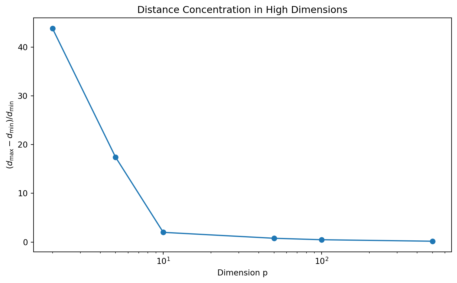
Another high-dimensional problem is distance concentration. In many high-dimensional settings, the nearest and farthest distance become similar. If all points are almost equally far away, the word “nearest” loses meaning.

One way to measure this is

\[ \frac{d_\max-d_\min}{d_\min} \]

where \(d_\min\) is the distance from a query point to its nearest neighbor and \(d_\max\) is the distance to its farthest neighbor. In high dimensions, this ratio often shrinks.

import numpy as np
import matplotlib.pyplot as plt

rng = np.random.default_rng(42)

dimensions = [2, 5, 10, 50, 100, 500]
ratios = []

for p in dimensions:
    X = rng.uniform(0, 1, size=(2000, p))
    query = rng.uniform(0, 1, size=(1, p))

    distances = np.sqrt(((X - query) ** 2).sum(axis=1))
    d_min = distances.min()
    d_max = distances.max()

    ratios.append((d_max - d_min) / d_min)

plt.figure(figsize=(8, 5))
plt.plot(dimensions, ratios, marker="o")
plt.title("Distance Concentration in High Dimensions")
plt.xlabel("Dimension p")
plt.ylabel(r"$(d_{\max}-d_{\min})/d_{\min}$")
plt.xscale("log")
plt.tight_layout()
plt.show()

Figure 6: Distance Concentration

8. Computation and Algoriths

8.1. Computational Cost of Naive KNN

For a single query point \(x\), brute-force KNN computes \(d(x, x_i)\) for all \(i=1,\dots, n\). If each distance computation costs

\[ O(p) \]

then the total cost per query is

\[ O(np) \]

For \(m\) query points, the cost is

$$

O(mnp)

$$

This can be expensive for large datasets.

Training cost is low because the algorithm mainly stores the data, so \(O(np)\) memory is required.

Thus, KNN has the opposite computational profile of many trained models:

Phase	KNN Cost
Training	Cheap
Prediction	Expensive
Memory	High

8.2. Accelerated Nearest Neighbor Search

To reduce prediction cost, implementations may use spatial indexing structures such as:

• k-d trees
• ball trees
• approximate nearest-neighbor indexes.

A k-d tree recursively partitions the feature space along coordinate axes. A ball tree partitions data into nested hyperspheres. These structure can speed up nearest-neighbor search in low or moderate dimensions. However, in high dimensions, their advantage often decreases because many branches must be searched.

Approximate nearest-neighbor methods trade exactness for speed. They are essential in large-scale applications such as image retrieval, recommender systems, vector databases, and semantic search.

8.3. Approximate Nearest Neighbors

Approximate nearest-neighbor methods seek a point \(\tilde x\) such that

\[ d(x, \tilde x) \leq (1+ \epsilon )\,d(x, x^*) \]

where \(x^*\) is the exact nearest neighbor and \(\epsilon >0\) controls approximation tolerance.

9. Advanced Extensions

9.1. Adaptive Nearest Neighbors

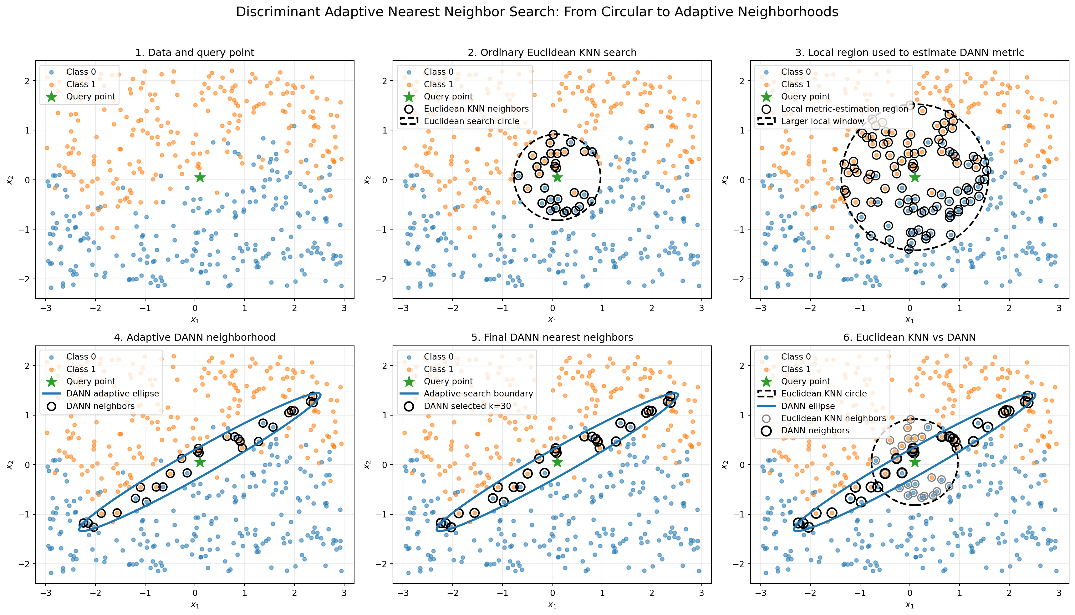
Ordinary KNN uses the same distance geometry throughout the feature space. But some regions may require elongated neighbors rather than spherical neighborhoods.

Discriminant Adaptive Nearest Neighborhood classification, or DANN, modifies the local metric using local class information. Hastie and Tibshirani proposed adapting nearest-neighbor neighborhoods to local class structure so that neighborhoods stretch in directions where class probabilities change slowly and shrink in directions where class probabilities change quickly².

The basic idea is to use a local metric

\[ d_A(x, z) = \sqrt{((x-z)^\top)A(x) (x-z)} \]

where \(A(x)\) is a positive semidefinite matrix adapted to the local neighborhood around \(x\).

If class boundaries vary sharply in one direction, \(A(x)\) can make distances grow faster in that direction. If class probabilities are stable in another direction, the metric can stretch the neighborhood in that direction. This reduces bias without necessarily increasing variance.

import numpy as np
import matplotlib.pyplot as plt
from matplotlib.patches import Circle

np.random.seed(42)

n = 450

x1 = np.random.uniform(-3, 3, n)
x2 = np.random.uniform(-2.2, 2.2, n)

# Curved class boundary
boundary = 0.75 * np.sin(1.2 * x1)

# Add noise so the local structure is not perfectly separable
noise = np.random.normal(0, 0.35, n)

y = (x2 + noise > boundary).astype(int)

X = np.column_stack([x1, x2])

# Query point where we want to classify a new observation
x_query = np.array([0.1, 0.05])

def euclidean_distances(X, x):
    return np.sqrt(np.sum((X - x) ** 2, axis=1))


def knn_indices_euclidean(X, x, k):
    d = euclidean_distances(X, x)
    return np.argsort(d)[:k], d


def inverse_square_root_matrix(M, eps=1e-6):
    """
    Compute M^{-1/2} for a symmetric positive semidefinite matrix.
    """
    eigvals, eigvecs = np.linalg.eigh(M)

    eigvals = np.maximum(eigvals, eps)

    D_inv_sqrt = np.diag(1.0 / np.sqrt(eigvals))

    return eigvecs @ D_inv_sqrt @ eigvecs.T


def estimate_dann_metric(X_local, y_local, ridge=1e-3, epsilon=0.05):
    """
    Estimate a simplified DANN local metric.

    W = local within-class covariance
    B = local between-class covariance

    A = W^{-1/2} (W^{-1/2} B W^{-1/2} + epsilon I) W^{-1/2}

    Larger distance growth occurs in locally discriminative directions.
    """

    n_local, p = X_local.shape

    overall_mean = X_local.mean(axis=0)

    W = np.zeros((p, p))
    B = np.zeros((p, p))

    for c in np.unique(y_local):
        X_c = X_local[y_local == c]
        n_c = len(X_c)

        mean_c = X_c.mean(axis=0)

        centered_c = X_c - mean_c
        W += centered_c.T @ centered_c

        mean_diff = (mean_c - overall_mean).reshape(-1, 1)
        B += n_c * (mean_diff @ mean_diff.T)

    W = W / n_local
    B = B / n_local

    # Regularization for numerical stability
    W = W + ridge * np.eye(p)

    W_inv_sqrt = inverse_square_root_matrix(W)

    B_tilde = W_inv_sqrt @ B @ W_inv_sqrt

    A = W_inv_sqrt @ (B_tilde + epsilon * np.eye(p)) @ W_inv_sqrt

    return A, W, B


def metric_distances(X, x, A):
    diffs = X - x
    return np.sqrt(np.sum((diffs @ A) * diffs, axis=1))


def ellipse_from_metric(x_center, A, radius, n_points=250):
    """
    Plot the contour:

        (z - x)^T A (z - x) = radius^2

    This is an ellipse when A is positive definite.
    """

    eigvals, eigvecs = np.linalg.eigh(A)

    eigvals = np.maximum(eigvals, 1e-8)

    theta = np.linspace(0, 2 * np.pi, n_points)

    unit_circle = np.column_stack([np.cos(theta), np.sin(theta)])

    axes_lengths = radius / np.sqrt(eigvals)

    ellipse = unit_circle @ np.diag(axes_lengths) @ eigvecs.T

    return ellipse + x_center


def majority_vote(y_neighbors):
    values, counts = np.unique(y_neighbors, return_counts=True)
    return values[np.argmax(counts)]

k_final = 30       # final number of neighbors
m_local = 100      # larger local neighborhood used to estimate local metric

# ordinary Euclidean KNN
idx_knn, d_euclid = knn_indices_euclidean(X, x_query, k_final)

# larger Euclidean neighborhood for estimating local class structure
idx_local, _ = knn_indices_euclidean(X, x_query, m_local)

X_local = X[idx_local]
y_local = y[idx_local]

# estimate the DANN local metric
A, W, B = estimate_dann_metric(X_local, y_local)

# use adaptive metric to search for nearest neighbors
d_dann = metric_distances(X, x_query, A)
idx_dann = np.argsort(d_dann)[:k_final]

# Radius of ordinary KNN circle
r_knn = d_euclid[idx_knn[-1]]

# Radius of DANN adaptive ellipse
r_dann = d_dann[idx_dann[-1]]

ellipse_dann = ellipse_from_metric(x_query, A, r_dann)

# Predictions
pred_knn = majority_vote(y[idx_knn])
pred_dann = majority_vote(y[idx_dann])

print("Euclidean KNN prediction:", pred_knn)
print("DANN prediction:", pred_dann)
print()
print("Local DANN metric A:")
print(A)

Euclidean KNN prediction: 0
DANN prediction: 1

Local DANN metric A:
[[ 2.45785784 -4.17558994]
 [-4.17558994  7.45534753]]

fig, axes = plt.subplots(2, 3, figsize=(18, 10))

axes = axes.ravel()

titles = [
    "1. Data and query point",
    "2. Ordinary Euclidean KNN search",
    "3. Local region used to estimate DANN metric",
    "4. Adaptive DANN neighborhood",
    "5. Final DANN nearest neighbors",
    "6. Euclidean KNN vs DANN"
]

for ax, title in zip(axes, titles):
    ax.scatter(X[y == 0, 0], X[y == 0, 1], s=20, alpha=0.55, label="Class 0")
    ax.scatter(X[y == 1, 0], X[y == 1, 1], s=20, alpha=0.55, label="Class 1")

    ax.scatter(
        x_query[0],
        x_query[1],
        s=180,
        marker="*",
        label="Query point",
        zorder=5
    )

    ax.set_title(title)
    ax.set_xlabel("$x_1$")
    ax.set_ylabel("$x_2$")
    ax.set_xlim(-3.2, 3.2)
    ax.set_ylim(-2.4, 2.4)
    ax.grid(alpha=0.25)

axes[0].legend(loc="upper left")

axes[1].scatter(
    X[idx_knn, 0],
    X[idx_knn, 1],
    s=90,
    facecolors="none",
    edgecolors="black",
    linewidths=1.7,
    label="Euclidean KNN neighbors"
)

circle = Circle(
    x_query,
    r_knn,
    fill=False,
    linewidth=2,
    linestyle="--",
    label="Euclidean search circle"
)

axes[1].add_patch(circle)
axes[1].legend(loc="upper left")

axes[2].scatter(
    X_local[:, 0],
    X_local[:, 1],
    s=100,
    facecolors="none",
    edgecolors="black",
    linewidths=1.4,
    label="Local metric-estimation region"
)

circle_local = Circle(
    x_query,
    euclidean_distances(X, x_query)[idx_local[-1]],
    fill=False,
    linewidth=2,
    linestyle="--",
    label="Larger local window"
)

axes[2].add_patch(circle_local)
axes[2].legend(loc="upper left")

axes[3].plot(
    ellipse_dann[:, 0],
    ellipse_dann[:, 1],
    linewidth=2.5,
    label="DANN adaptive ellipse"
)

axes[3].scatter(
    X[idx_dann, 0],
    X[idx_dann, 1],
    s=90,
    facecolors="none",
    edgecolors="black",
    linewidths=1.7,
    label="DANN neighbors"
)

axes[3].legend(loc="upper left")

axes[4].plot(
    ellipse_dann[:, 0],
    ellipse_dann[:, 1],
    linewidth=2.5,
    label="Adaptive search boundary"
)

axes[4].scatter(
    X[idx_dann, 0],
    X[idx_dann, 1],
    s=110,
    facecolors="none",
    edgecolors="black",
    linewidths=1.9,
    label=f"DANN selected k={k_final}"
)

axes[4].legend(loc="upper left")

circle_compare = Circle(
    x_query,
    r_knn,
    fill=False,
    linewidth=2,
    linestyle="--",
    label="Euclidean KNN circle"
)

axes[5].add_patch(circle_compare)

axes[5].plot(
    ellipse_dann[:, 0],
    ellipse_dann[:, 1],
    linewidth=2.5,
    label="DANN ellipse"
)

axes[5].scatter(
    X[idx_knn, 0],
    X[idx_knn, 1],
    s=80,
    facecolors="none",
    edgecolors="gray",
    linewidths=1.4,
    label="Euclidean KNN neighbors"
)

axes[5].scatter(
    X[idx_dann, 0],
    X[idx_dann, 1],
    s=130,
    facecolors="none",
    edgecolors="black",
    linewidths=1.9,
    label="DANN neighbors"
)

axes[5].legend(loc="upper left")

fig.suptitle(
    "Discriminant Adaptive Nearest Neighbor Search: From Circular to Adaptive Neighborhoods",
    fontsize=16,
    y=1.02
)

plt.tight_layout()
plt.show()

Ordinary KNN searches using a circular neighborhood because all directions are treated equally.

DANN first looks at a larger local region around the query point and estimates the directions in which the class labels change most strongly.

The final neighborhood becomes elliptical: it shrinks in directions where class probabilities change quickly and stretches in directions where class probabilities are relatively stable.

Therefore, DANN can choose neighbors that are more consistent with the local class boundary than ordinary Euclidean KNN.

9.2. Tangent Distance KNN

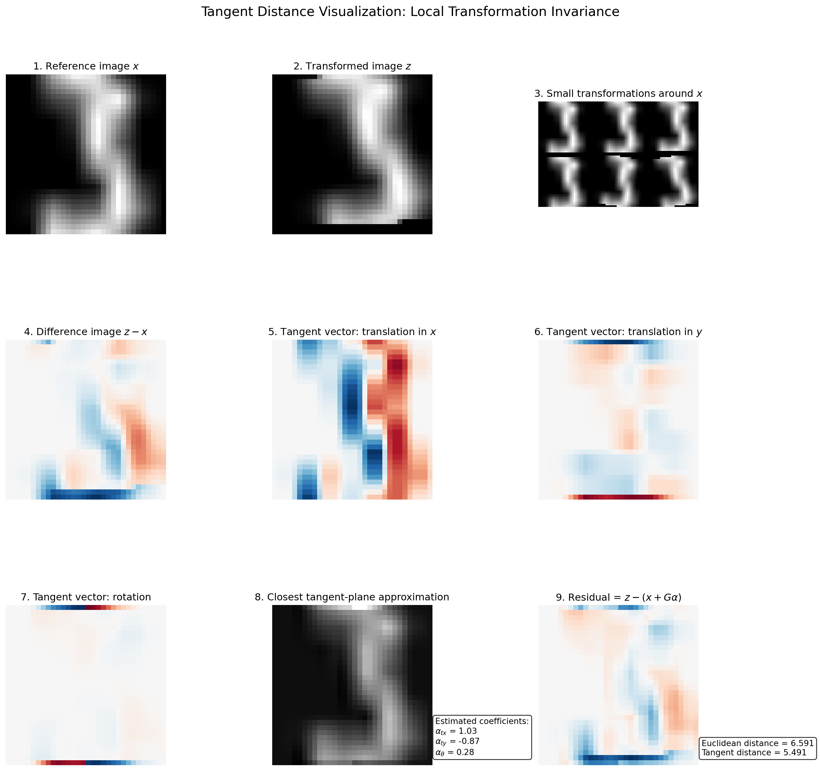
In image recognition, two images of the same object may differ by small transformations: translation, rotation, scaling, or deformation. Ordinary Euclidean distance between raw pixels may treat these as large differences even though the semantic object is unchanged.

Tangent distance addresses this by measuring distance between transformation manifolds rather than raw images. Suppose an image is represented as a vector \(x\in \mathbb R^p\). Let \(\mathcal M_x\) be the manifold of small transformations of \(x\), such as small rotations or translations. Tangent distance approximates this manifold locally by a tangent plane.

Instead of comparing \(||x-z||_2\), one compares the distance between local tangent approximations of \(\mathcal M_x\) and \(\mathcal M_z\).

import numpy as np
import matplotlib.pyplot as plt

from sklearn.datasets import load_digits
from scipy.ndimage import rotate, shift, zoom

digits = load_digits()

idx = np.where(digits.target == 3)[0][5]

x_small = digits.images[idx]              # original 8x8 digit
x_small = x_small / x_small.max()         # normalize to [0,1]

x = zoom(x_small, 4, order=1)             # now about 32x32
x = np.clip(x, 0, 1)

print("Image shape:", x.shape)

Image shape: (32, 32)

def normalize_img(img):
    img = img - img.min()
    if img.max() > 0:
        img = img / img.max()
    return img

def transform_image(img, tx=0.0, ty=0.0, theta=0.0):
    """
    Apply a small rotation and translation.
    tx = horizontal shift (pixels)
    ty = vertical shift (pixels)
    theta = rotation angle in degrees
    """
    out = rotate(img, angle=theta, reshape=False, order=1, mode="constant", cval=0.0)
    out = shift(out, shift=(ty, tx), order=1, mode="constant", cval=0.0)
    return np.clip(out, 0, 1)

def tangent_vector(img, param="tx", delta=1.0):
    """
    Finite-difference approximation of tangent vectors:
        dT/dtx, dT/dty, dT/dtheta
    """
    if param == "tx":
        plus  = transform_image(img, tx= delta, ty=0.0, theta=0.0)
        minus = transform_image(img, tx=-delta, ty=0.0, theta=0.0)
        vec = (plus - minus) / (2 * delta)

    elif param == "ty":
        plus  = transform_image(img, tx=0.0, ty= delta, theta=0.0)
        minus = transform_image(img, tx=0.0, ty=-delta, theta=0.0)
        vec = (plus - minus) / (2 * delta)

    elif param == "theta":
        plus  = transform_image(img, tx=0.0, ty=0.0, theta= delta)
        minus = transform_image(img, tx=0.0, ty=0.0, theta=-delta)
        vec = (plus - minus) / (2 * delta)

    else:
        raise ValueError("param must be one of: 'tx', 'ty', 'theta'")

    return vec

def make_montage(images, nrows, ncols, pad=2, pad_value=0.0):
    """
    Arrange a list of images into a simple montage.
    """
    h, w = images[0].shape
    canvas = np.full(
        (nrows * h + (nrows - 1) * pad, ncols * w + (ncols - 1) * pad),
        pad_value
    )

    for k, img in enumerate(images):
        r = k // ncols
        c = k % ncols
        y0 = r * (h + pad)
        x0 = c * (w + pad)
        canvas[y0:y0+h, x0:x0+w] = img

    return canvas

# True small transformation used to create z
tx_true = 1.4
ty_true = -1.1
theta_true = 8.0

z = transform_image(x, tx=tx_true, ty=ty_true, theta=theta_true)

# Tangent vectors at x
t_tx = tangent_vector(x, param="tx", delta=1.0)
t_ty = tangent_vector(x, param="ty", delta=1.0)
t_th = tangent_vector(x, param="theta", delta=1.0)

# Difference between the transformed image and the base image
d = (z - x).ravel()

# Build tangent basis matrix
G = np.column_stack([
    t_tx.ravel(),
    t_ty.ravel(),
    t_th.ravel()
])

# Least-squares projection of (z - x) onto tangent space at x
alpha, _, _, _ = np.linalg.lstsq(G, d, rcond=None)

# Closest point on the tangent plane
x_tangent_approx = x + (G @ alpha).reshape(x.shape)

# Residual after tangent-plane approximation
residual = z - x_tangent_approx

# Distances
euclidean_distance = np.linalg.norm((z - x).ravel())
tangent_distance = np.linalg.norm(residual.ravel())

print("Estimated tangent coefficients [tx, ty, theta]:")
print(alpha)
print()
print(f"Euclidean distance between x and z: {euclidean_distance:.4f}")
print(f"Tangent distance between x and z:  {tangent_distance:.4f}")

Estimated tangent coefficients [tx, ty, theta]:
[ 1.02679049 -0.86907804  0.28039056]

Euclidean distance between x and z: 6.5915
Tangent distance between x and z:  5.4914

samples = [
    transform_image(x, tx=-1.0, ty=0.0, theta=0.0),
    transform_image(x, tx= 1.0, ty=0.0, theta=0.0),
    transform_image(x, tx=0.0, ty=-1.0, theta=0.0),
    transform_image(x, tx=0.0, ty= 1.0, theta=0.0),
    transform_image(x, tx=0.0, ty=0.0, theta=-8.0),
    transform_image(x, tx=0.0, ty=0.0, theta= 8.0),
]

sample_titles = [
    "tx=-1", "tx=+1",
    "ty=-1", "ty=+1",
    "rot=-8°", "rot=+8°"
]

montage = make_montage(samples, nrows=2, ncols=3, pad=2, pad_value=0.0)

fig, axes = plt.subplots(3, 3, figsize=(14, 14))
axes = axes.ravel()

axes[0].imshow(x, cmap="gray")
axes[0].set_title("1. Reference image $x$")
axes[0].axis("off")

axes[1].imshow(z, cmap="gray")
axes[1].set_title("2. Transformed image $z$")
axes[1].axis("off")

axes[2].imshow(montage, cmap="gray")
axes[2].set_title("3. Small transformations around $x$")
axes[2].axis("off")

vmax_diff = np.max(np.abs(z - x))
axes[3].imshow(z - x, cmap="RdBu_r", vmin=-vmax_diff, vmax=vmax_diff)
axes[3].set_title("4. Difference image $z - x$")
axes[3].axis("off")

vmax_tx = np.max(np.abs(t_tx))
axes[4].imshow(t_tx, cmap="RdBu_r", vmin=-vmax_tx, vmax=vmax_tx)
axes[4].set_title("5. Tangent vector: translation in $x$")
axes[4].axis("off")

vmax_ty = np.max(np.abs(t_ty))
axes[5].imshow(t_ty, cmap="RdBu_r", vmin=-vmax_ty, vmax=vmax_ty)
axes[5].set_title("6. Tangent vector: translation in $y$")
axes[5].axis("off")

vmax_th = np.max(np.abs(t_th))
axes[6].imshow(t_th, cmap="RdBu_r", vmin=-vmax_th, vmax=vmax_th)
axes[6].set_title("7. Tangent vector: rotation")
axes[6].axis("off")

axes[7].imshow(x_tangent_approx, cmap="gray")
axes[7].set_title("8. Closest tangent-plane approximation")
axes[7].axis("off")

text8 = (
    f"Estimated coefficients:\n"
    f"$\\alpha_{{tx}}$ = {alpha[0]:.2f}\n"
    f"$\\alpha_{{ty}}$ = {alpha[1]:.2f}\n"
    f"$\\alpha_{{\\theta}}$ = {alpha[2]:.2f}"
)
axes[7].text(
    1.02, 0.05, text8,
    transform=axes[7].transAxes,
    fontsize=10,
    va="bottom",
    bbox=dict(boxstyle="round", facecolor="white", alpha=0.85)
)

vmax_res = np.max(np.abs(residual))
axes[8].imshow(residual, cmap="RdBu_r", vmin=-vmax_res, vmax=vmax_res)
axes[8].set_title("9. Residual = $z - (x + G\\alpha)$")
axes[8].axis("off")

text9 = (
    f"Euclidean distance = {euclidean_distance:.3f}\n"
    f"Tangent distance = {tangent_distance:.3f}"
)
axes[8].text(
    1.02, 0.05, text9,
    transform=axes[8].transAxes,
    fontsize=10,
    va="bottom",
    bbox=dict(boxstyle="round", facecolor="white", alpha=0.85)
)

fig.suptitle(
    "Tangent Distance Visualization: Local Transformation Invariance",
    fontsize=16,
    y=0.98
)

plt.tight_layout()
plt.show()

9.3. KNN Graphs

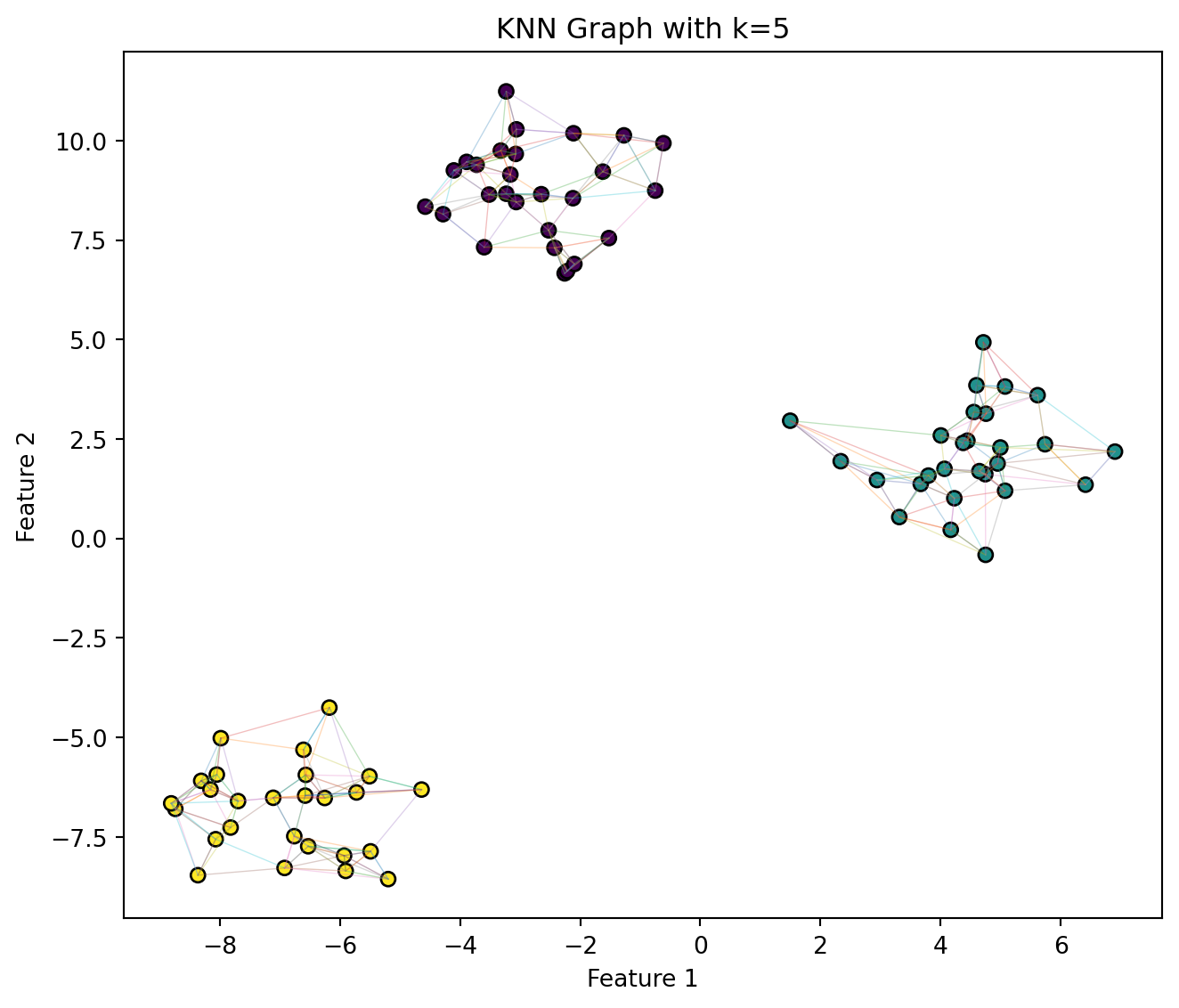
KNN also defines graphs. Given data points \(x_1, \dots, x_n,\) construct a graph \(G=(V,E),\) where \(V=\{1,\dots, n\}\). A directed edge exists from \(i\) to \(k\) if \(j\in N_k(x_i)\). This is called KNN Graph.

The adjacency matrix is

\[ A_{ij} =\begin{cases} 1, & j\in N_k(x_i)\\ 0, & \text{otherwise} \end{cases} \]

A weighted version is

\[ A_{ij} =\exp\left(-\frac{d(x_i,x_j)^2}{2h^2}\right)\mathbf{I}\{j\in N_k(x_i)\} \]

KNN graphs are used in:

• manifold learning.
• spectral clustering,
• semi-supervised learning,
• community detection,
• graph-based anomaly detection.

import numpy as np
import matplotlib.pyplot as plt
from sklearn.datasets import make_blobs
from sklearn.neighbors import kneighbors_graph

X, y = make_blobs(n_samples=80, centers=3, random_state=42, cluster_std=1.2)

A = kneighbors_graph(X, n_neighbors=5, mode="connectivity", include_self=False)
A = A.toarray()

plt.figure(figsize=(7, 6))

for i in range(X.shape[0]):
    for j in range(X.shape[0]):
        if A[i, j] == 1:
            plt.plot(
                [X[i, 0], X[j, 0]],
                [X[i, 1], X[j, 1]],
                linewidth=0.5,
                alpha=0.3
            )

plt.scatter(X[:, 0], X[:, 1], c=y, edgecolor="k")
plt.title("KNN Graph with k=5")
plt.xlabel("Feature 1")
plt.ylabel("Feature 2")
plt.tight_layout()
plt.show()

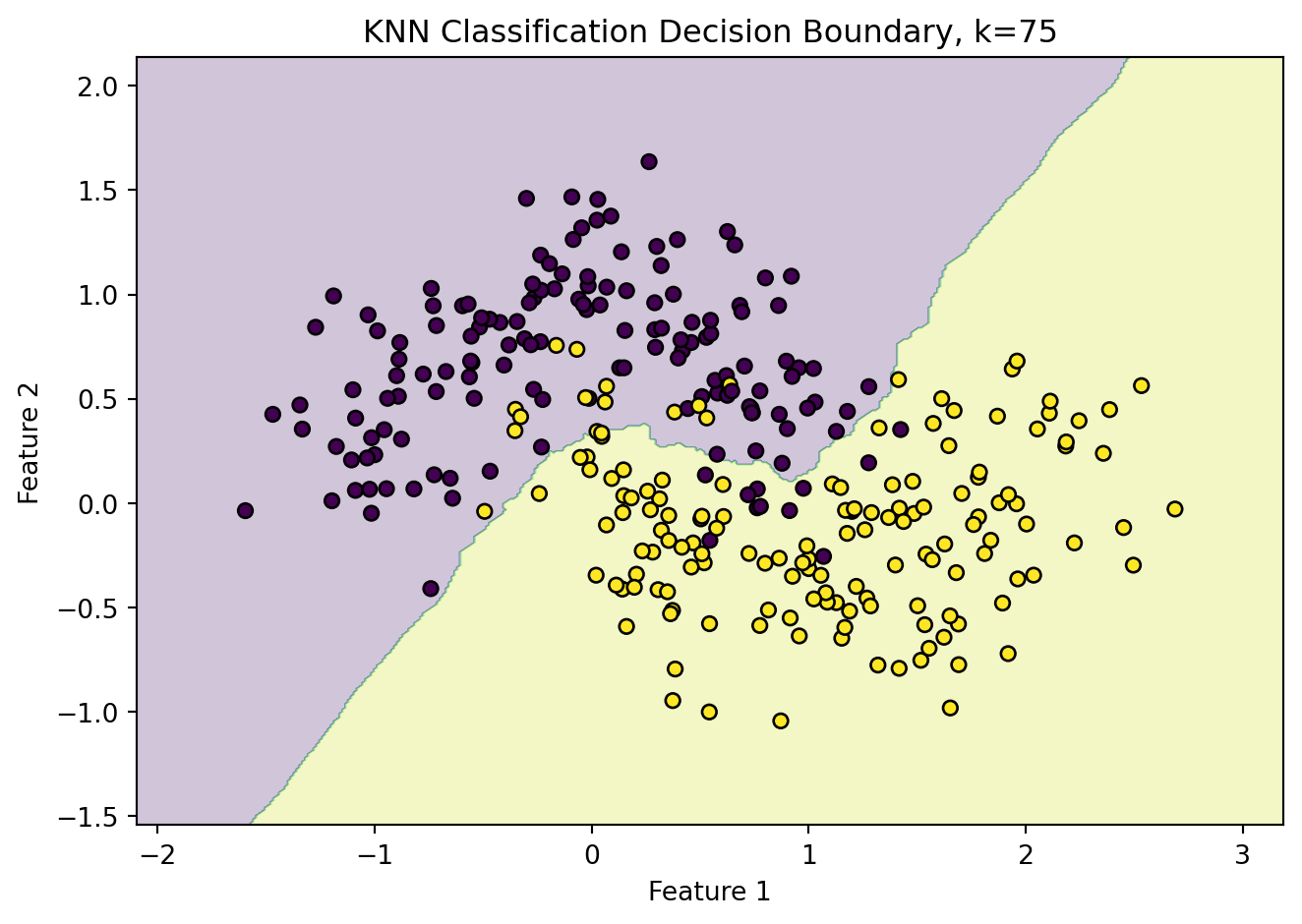
Figure 7: KNN Graph

10. Examples

10.1. Handwritten Digit Recognition

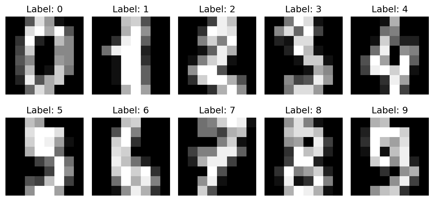
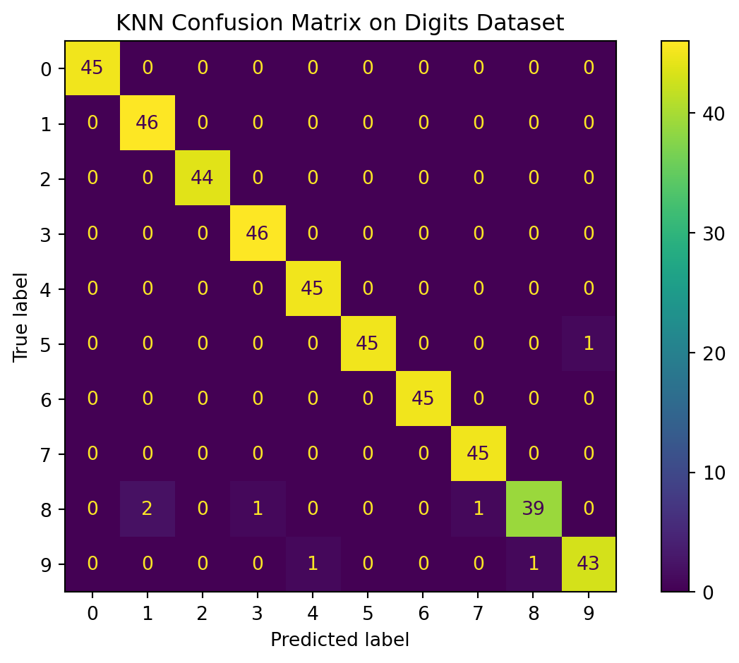
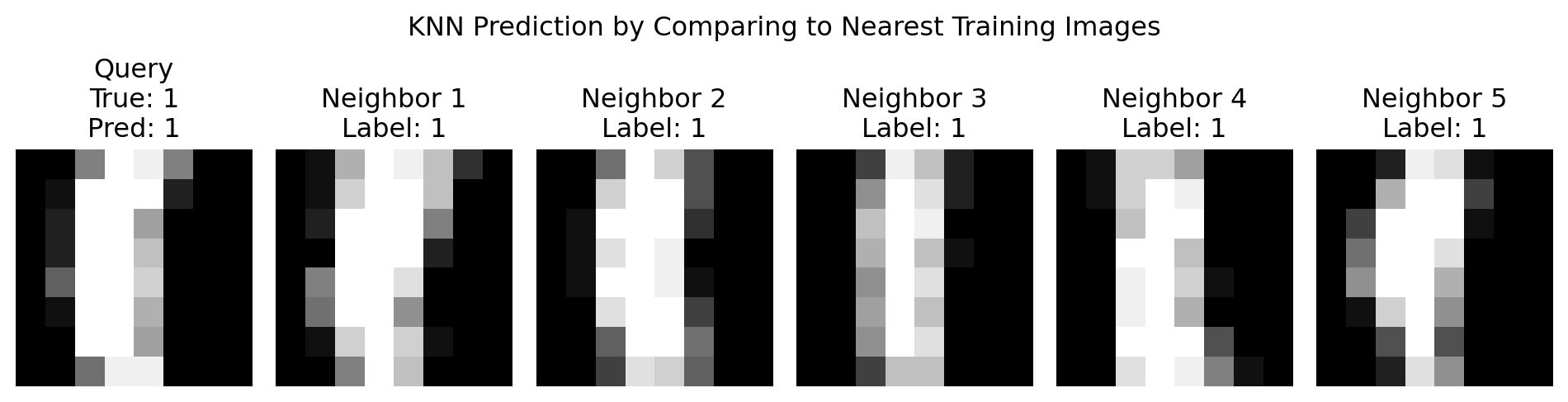
Handwritten digit recognition is a classical KNN application. Each image is represented as a vector of pixel intensities. A KNN classifier the digit by finding training images whose pixel patterns are closest to the query image.

Mathematically, each image is flattened into \(x_i\in \mathbb R^{64}\), and the label is \(y_i\in \{0, \dots, 9\}\). A KNN classifier predicts

\[ \hat y(x) = \arg \max_{c\in \{0,\dots, 9\}}\sum_{i\in N_k(x)}\mathbf{I}\{y_i=c\} \]

import numpy as np
import matplotlib.pyplot as plt
from sklearn.datasets import load_digits
from sklearn.neighbors import KNeighborsClassifier
from sklearn.model_selection import train_test_split
from sklearn.metrics import ConfusionMatrixDisplay, accuracy_score

digits = load_digits()

X = digits.data
y = digits.target
images = digits.images

plt.figure(figsize=(8, 4))
for i in range(10):
    plt.subplot(2, 5, i + 1)
    plt.imshow(images[i], cmap="gray")
    plt.title(f"Label: {y[i]}")
    plt.axis("off")
plt.tight_layout()
plt.show()

# Train-test split
X_train, X_test, y_train, y_test, images_train, images_test = train_test_split(
    X, y, images, test_size=0.25, random_state=42, stratify=y
)

knn = KNeighborsClassifier(n_neighbors=5)
knn.fit(X_train, y_train)

y_pred = knn.predict(X_test)
acc = accuracy_score(y_test, y_pred)

print("Test accuracy:", acc)

# Confusion matrix
ConfusionMatrixDisplay.from_predictions(y_test, y_pred)
plt.title("KNN Confusion Matrix on Digits Dataset")
plt.tight_layout()
plt.show()

# Show one query image and its nearest neighbors
query_index = 0
query = X_test[query_index].reshape(1, -1)

distances, indices = knn.kneighbors(query, n_neighbors=5)

plt.figure(figsize=(10, 3))

plt.subplot(1, 6, 1)
plt.imshow(images_test[query_index], cmap="gray")
plt.title(f"Query\nTrue: {y_test[query_index]}\nPred: {knn.predict(query)[0]}")
plt.axis("off")

for rank, idx in enumerate(indices[0]):
    plt.subplot(1, 6, rank + 2)
    plt.imshow(images_train[idx], cmap="gray")
    plt.title(f"Neighbor {rank+1}\nLabel: {y_train[idx]}")
    plt.axis("off")

plt.suptitle("KNN Prediction by Comparing to Nearest Training Images")
plt.tight_layout()
plt.show()

Test accuracy: 0.9844444444444445

10.2. Recommender Systems

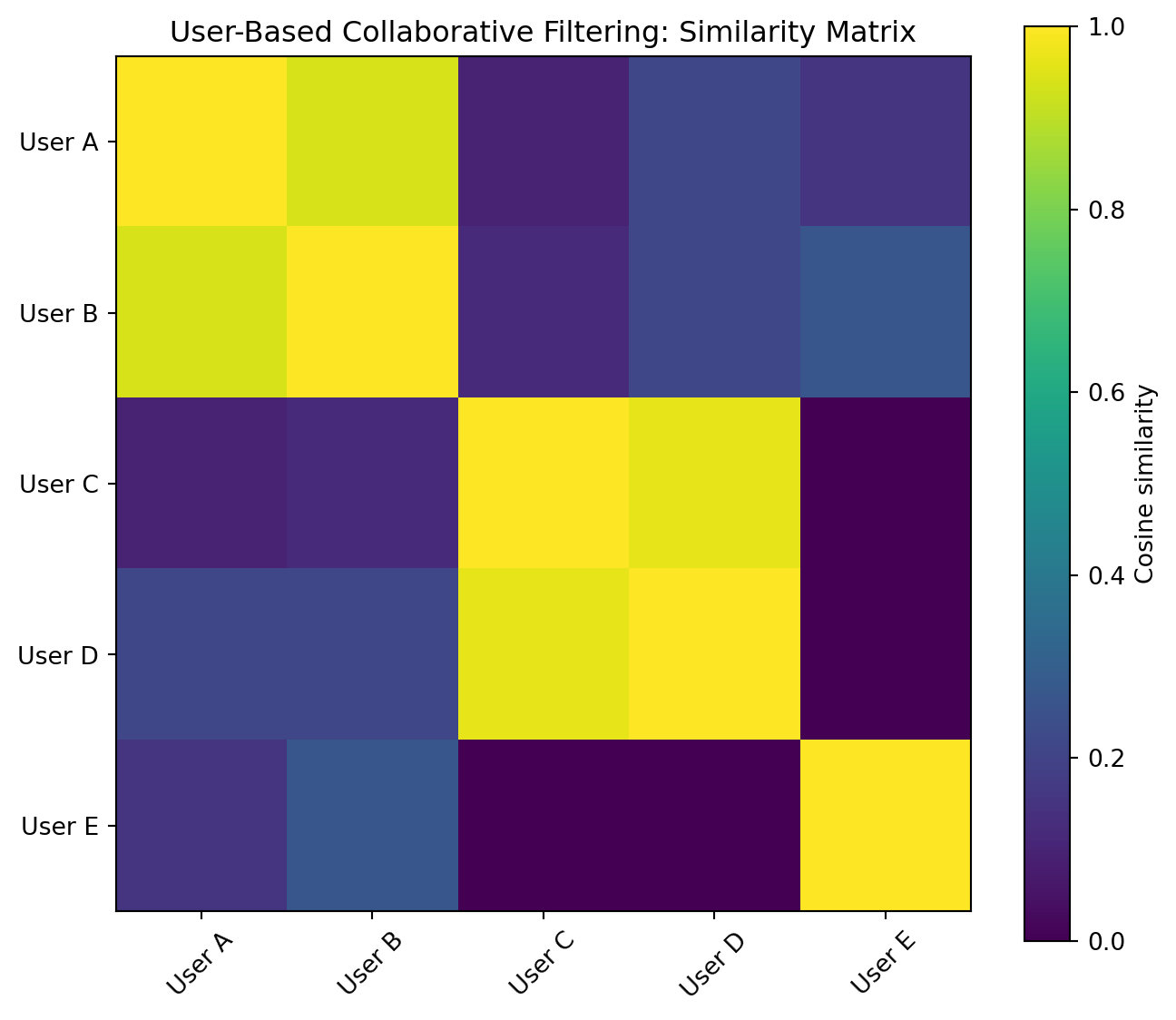
In collaborative filtering, KNN can recommend items by finding similar users or similar items. Let \(R\in \mathbb R^{m\times q}\) be a user-item rating matrix, where \(R_{ui}\) is the rating given by user \(u\) to item \(i\).

In user-based collaborative filtering, the similarity between users \(u\) and \(v\) may be computed using cosine similarity

\[ s(u,v) = \frac{R_u^\top R_v}{||R_u||_2 ||R_v||_2} \]

The predicted rating of user \(u\) for item \(i\) is

\[ \hat R_{ui} = \frac{\sum_{v\in N_k(u)}s(u,v)R_{vi}}{\sum_{v\in N_k(u)}|s(u,v)|} \]

In words, a user’s rating is predicted by averaging ratings from similar users, weighted by similarity.

import numpy as np
import pandas as pd
import matplotlib.pyplot as plt
from sklearn.metrics.pairwise import cosine_similarity

ratings = pd.DataFrame({
    "Action Movie": [5, 4, 0, 0, 1],
    "Comedy Movie": [4, 5, 0, 1, 0],
    "Horror Movie": [0, 1, 5, 4, 0],
    "Sci-Fi Movie": [1, 0, 4, 5, 0],
    "Romance Movie": [0, 1, 0, 0, 5],
}, index=["User A", "User B", "User C", "User D", "User E"])

similarity = cosine_similarity(ratings)

plt.figure(figsize=(7, 6))
plt.imshow(similarity)
plt.colorbar(label="Cosine similarity")
plt.xticks(range(len(ratings.index)), ratings.index, rotation=45)
plt.yticks(range(len(ratings.index)), ratings.index)
plt.title("User-Based Collaborative Filtering: Similarity Matrix")
plt.tight_layout()
plt.show()

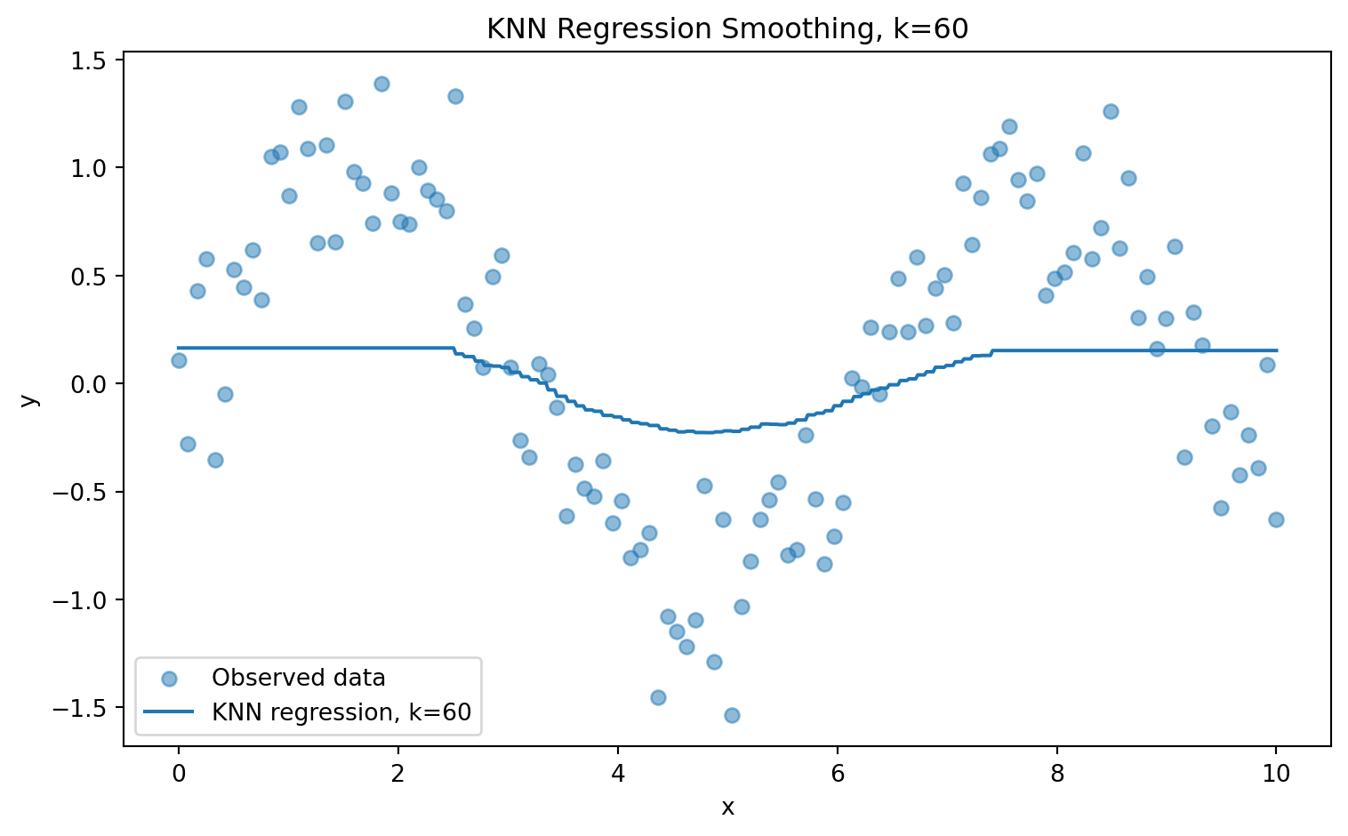
Figure 8: User Similarity Heatmap

10.3. Anomaly Detection

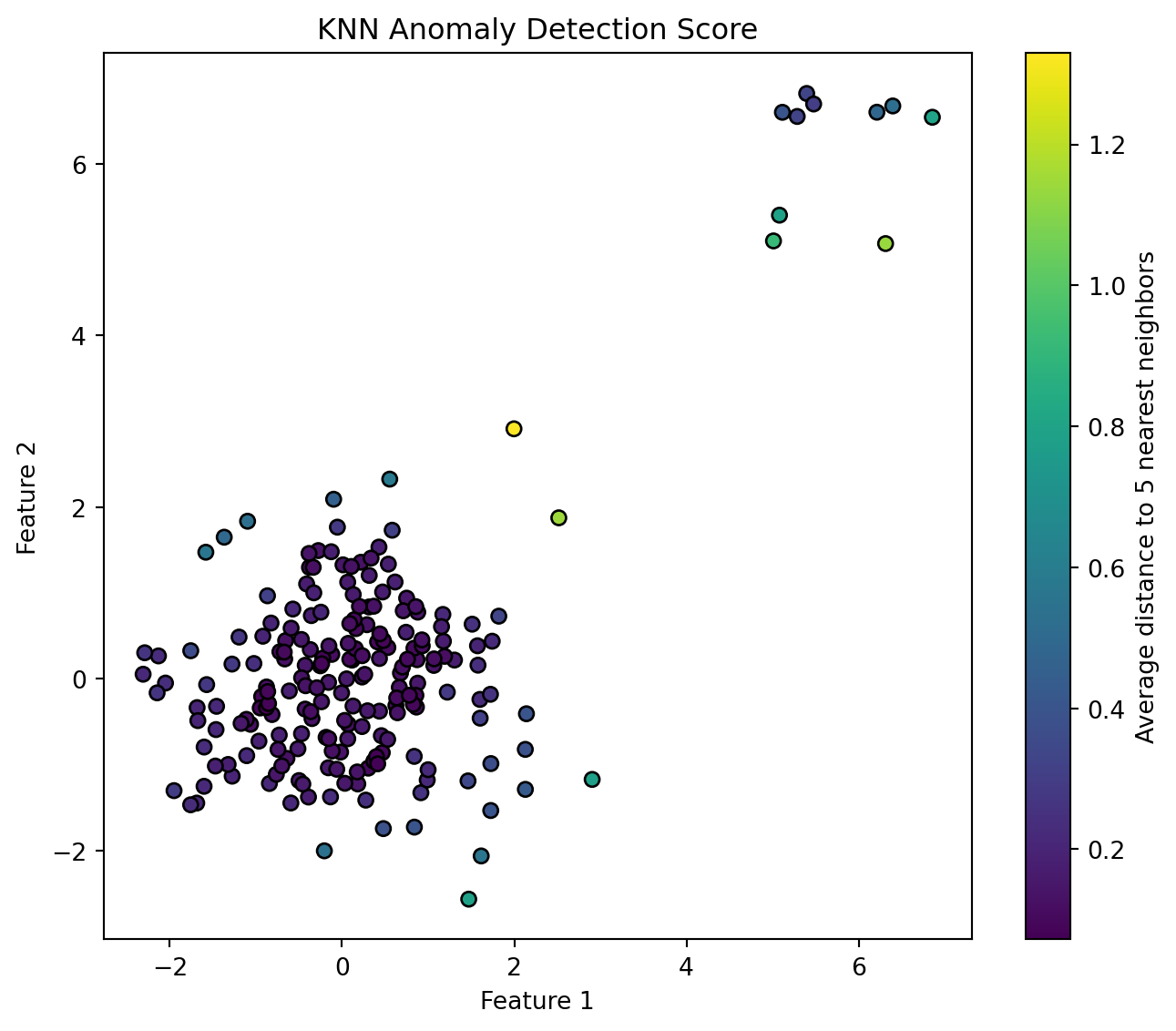
KNN can also be used for anomaly detection. The idea is that normal points lie close to many other points, while anomalies are far from their neighbors.

Define the KNN anomaly score as the average distance to the \(k\) nearest neighbors:

\[ A_k(x) = \frac{1}{k}\sum_{i\in N_k(x)}d(x, x_i) \]

Large values of \(A_k(x)\) indicate that \(x\) is isolated.

import numpy as np
import matplotlib.pyplot as plt
from sklearn.neighbors import NearestNeighbors

rng = np.random.default_rng(42)

normal = rng.normal(0, 1, size=(200, 2))
anomalies = rng.uniform(5, 7, size=(10, 2))

X = np.vstack([normal, anomalies])

nn = NearestNeighbors(n_neighbors=5)
nn.fit(X)

distances, indices = nn.kneighbors(X)
scores = distances.mean(axis=1)

plt.figure(figsize=(7, 6))
plt.scatter(X[:, 0], X[:, 1], c=scores, edgecolor="k")
plt.colorbar(label="Average distance to 5 nearest neighbors")
plt.title("KNN Anomaly Detection Score")
plt.xlabel("Feature 1")
plt.ylabel("Feature 2")
plt.tight_layout()
plt.show()

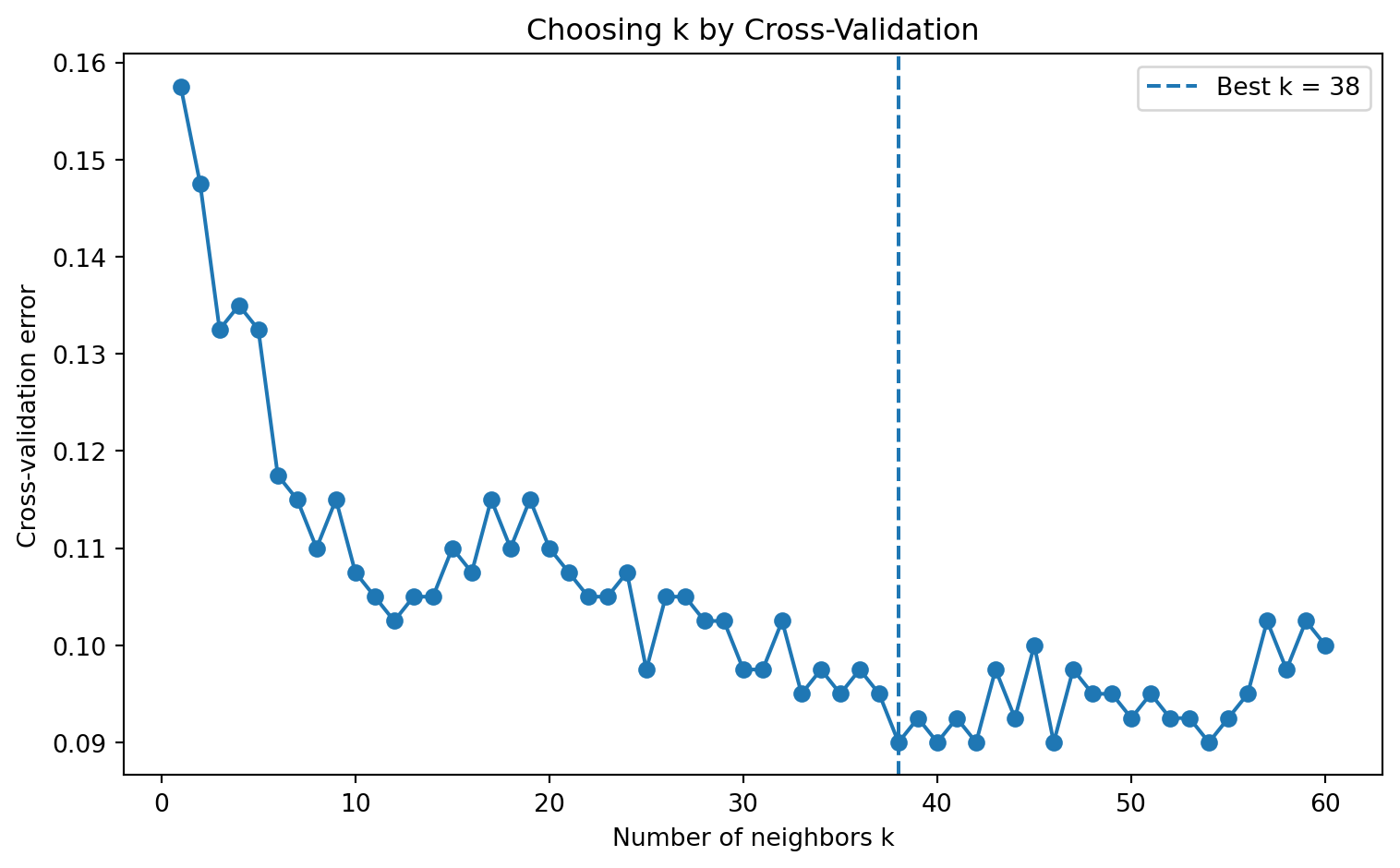
Figure 9: Anomaly Detection

---

K-Nearest Neighbors is one of the simplest and most important models in supervised learning. Its central principle is local similarity: to predict the response for a new point, inspect the most similar points already observed.

Mathematically, KNN replaces global model fitting with local neighborhood estimation. For classification, it estimates local class probabilities through neighbor voting. For regression, it estimates the conditional mean through local averaging. Its behavior is controlled primarily by the distance metric and the number of neighbors \(k\).

KNN is powerful because it is flexible, intuitive, and non-parametric. It can model nonlinear boundaries without explicitly fitting a nonlinear equation. It can be extended to weighted voting, adaptive metrics, tangent distances, approximate search, anomaly detection, recommender systems, and graph-based learning.

At the same time, KNN has serious limitations. Its dependence on distance makes it sensitive to scaling, irrelevant variables, and high dimensionality. Its memory-based nature makes prediction expensive for large datasets. Its local averaging structure means it usually cannot extrapolate.

Next chapter: Data Modeling - SVM

---

Footnotes

1. Cover, T., and P. Hart. “Nearest Neighbor Pattern Classification.” IEEE Transactions on Information Theory 13, no. 1 (1967): 21–27. https://doi.org/10.1109/TIT.1967.1053964.

2. Hastie, T., and R. Tibshirani. “Discriminant Adaptive Nearest Neighbor Classification.” IEEE Transactions on Pattern Analysis and Machine Intelligence 18, no. 6 (1996): 607–16. https://doi.org/10.1109/34.506411.