Data Science, Data Mining, and the Process of Turning Data into Knowledge
1. Introduction: What is Data Science?
Data science can be understood as the modern practice of applying the scientific method to data through computation. Its purpose is not merely to collect data, summarize, or build software systems, but to transform raw observations into reliable explanations, predictions, and decisions. In this sense, data science is both a technical discipline and an applied problem-solving framework. It combines statistical reasoning, computation implementation, and domain knowledge in order to extract useful information from complex data.
The rise of data science did not happen suddenly. Its intellectual roots can be traced to earlier discussions about “data analysis” as a field in its own right. John Tukey argued in 1962 that data analysis deserved recognition as more than a branch of mathematical statistics; it was a practical science concerned with learning from data1. Later, William Cleveland proposed expanding statistics into what he called data science, emphasizing computation, models, applications, pedagogy, and tools for practicing data analysts2. David Donoho later described the modern data science movement as part of a longer historical trajectory that includes statistics, computation, visualization, machine learning, and reproducible research3.
NoteDefinition
Data science is the interdisciplinary process of using data, computation, statistical reasoning, and domain knowledge to understand phenomena, make predictions, and support decisions.
This definition is intentionally broad. A data scientist may use regression models, neural networks, visualization, databases, simulation, causal reasoning, or cloud-based pipelines. What unifies these activities is the goal: to convert data into knowledge that can be evaluated, communicated, and used.
2. The Interdisciplinary Nature of Data Science
A common way to explain data science is through three overlapping skill areas: data analysis, software engineering, and domain expertise.
2.1. Data Analysis
The first dimension is data analysis. This includes descriptive statistics, visualization, statistical inference, machine learning, predictive modeling, uncertainty quantification, and evaluation. A data scientist must know how to ask questions such as:
What patterns are visible in the data?
Which variables appear to be associated?
Can we predicted an outcome accurately?
How uncertain are the predictions?
Are the observed relationships meaningful or accidental?
Does the model generalize to unseen data? Data analysis provides the scientific and mathematical foundation of data science. Without it, data science becomes a collection of software tools without a reliable way to judge truth, uncertainty, or error.
2.2. Software Engineering
The second dimension is software engineering. Real data science rarely happens in perfectly-clean textbook datasets. Data must be collected, stored, queried, cleaned, transformed, merged, modeled, visualized, and deployed. These tasks require programming ability and system-level thinking.
Software engineering matters because data science is often performed at scale. A model that works on a small CSV file may fail when applied to millions of records, streaming data, distributed databases, or production systems. Therefore, data scientists must often understand some (programming) languages such as Python, R, SQL, or Julia; tools for data pipelines; version control; reproducibility; and computational efficiency.
This is one reason data science differs from traditional statistical analysis. The data scientist is not only concerned with the mathematical validity of a model, but also with whether the full computational workflow can be reproduced, maintained, scaled, and deployed.
2.3. Domain Expertise
The third dimension is domain expertise. Data do not explain themselves. A dataset about hospital patients, airline delays, financial transactions, customer behavior, or climate observations requires contextual understanding. Domain expertise helps the data scientist formulate meaningful questions, define correct target variables, identify impossible values, interpret model results, or even decide predictions make practical sense.
For example, a model may discover that a certain medical treatment is associated with worse patient outcomes. Without medical knowledge, one might incorrectly conclude that the treatment causes harm. However, the treatment may be given only to the most severe patients. In this case, the apparent relationship reflects selection bias or confounding rather than a simple causal effect. Domain expertise is necessary to avoid such mistakes.
Thus, data science sits at the intersection of three forms of knowledge:
A strong data science requires all three. A technical elegant model may be useless if it answers the wrong question. A meaningful question may remain unanswered if the data pipeline is broken. A large dataset may produce misleading results if the analysis ignore bias, missingness, or uncertainty.
3. Data Mining and Knowledge Discovery
The term data mining is often used alongside data science. In everyday usage, data mining may refer to finding useful patterns in data. However, in the classical Knowledge Discovery in Databases literature, data mining has a more specific meaning. Fayyad, Piatetsky, Piatetsky-Shapiro, and Smyth define Knowledge Discovery in Databases, or KDD, as the broader of discovering useful knowledge from data, while data mining is the algorithmic step within that larger process where patterns or models are extracted4.
This distinction is important. Data mining is not the entire data science process. It is one part of it. Before mining patterns, the data scientist must understand the problem, select data, clean the data, transform variables, and decide what type of pattern would be useful. After mining patterns, the data scientist must evaluate them, interpret them, and determine whether they should be used in practice.
NoteDistinction
KDD/Data science process: The full workflow from problem formulation to deployed knowledge.
Data mining: The modeling or pattern-discovery stage inside that workflow.
TipExample
Suppose a retail company wants to identify customers likely to buy a new product. The data mining step might involve training a classification model. But the broader data science process includes defining what “likely to buy” means, selecting customer records, cleaning missing values, engineering behavior features, evaluating performance, explaining the model to marketing teams, and monitoring the model after deployment.
4. The Data Science Cycle
Data science is often mistakenly described as a linear sequence: collect data, clean data, train a model, deploy it. In practice, the process is iterative. A visualization may reveal missing values, forcing the analyst to revisit data collection. A model may perform poorly, forcing new feature engineering. Deployment may expose changing data patterns, requiring model retraining.
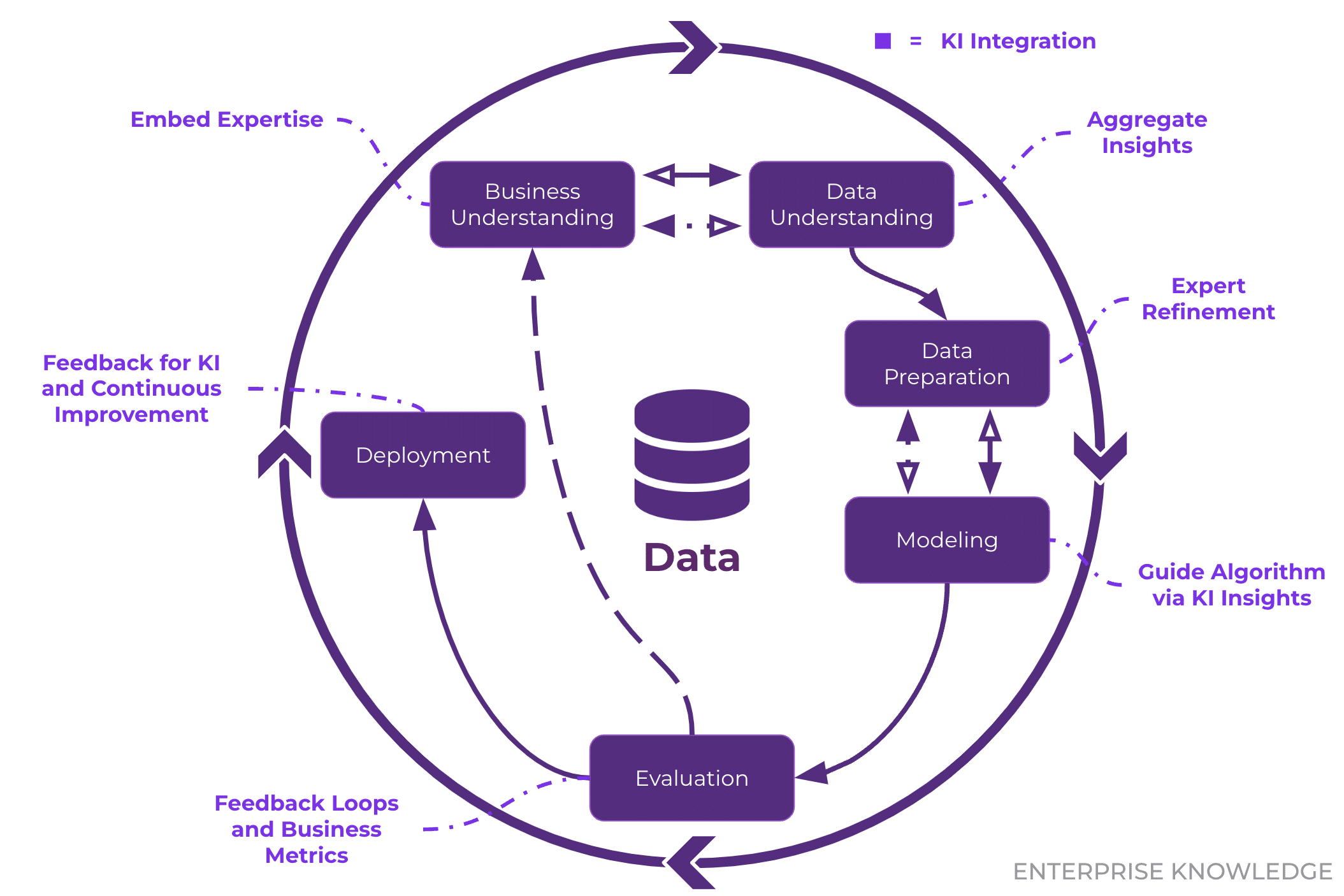
The CRISP-DM framework, one of the most widely cited process models for data mining projects, organizes the life cycle into six phases: business understanding, data understanding, data preparation, modeling, evaluation, and deployment. These phases are not linear; feedback loops are expected.
CRISP-DM framework
From my perspective, the process can be presented in the following expanded form:
Show code
flowchart LRA[Problem formulation] --> B[Data capture and selection] B --> C[Data understanding and exploratory analysis] C --> D[Data preparation and preprocessing] D --> E[Transformation and feature engineering] E --> F[Modeling and data mining] F --> G[Evaluation and interpretation] G --> H[Deployment and decision support] H --> I[Monitoring, feedback, and revision] I --> A C --> BG --> F
flowchart LR
A[Problem formulation] --> B[Data capture and selection]
B --> C[Data understanding and exploratory analysis]
C --> D[Data preparation and preprocessing]
D --> E[Transformation and feature engineering]
E --> F[Modeling and data mining]
F --> G[Evaluation and interpretation]
G --> H[Deployment and decision support]
H --> I[Monitoring, feedback, and revision]

I --> A
C --> B
G --> F
The first stage of data science is not data collection. We have to define the problem first. Before building a dataset or choosing an algorithm, the data scientist must define the question.
A weak question is vague:
“Can we use data to improve sales?”
A stronger data science question is operational:
“Can we predict, at the time of first customer inquiry, whether a customer is likely to purchase a new car within the next 30 days?”
The second question is better because it defines the unit of analysis, prediction target, time horizon, and decision context. It also suggests what data might be needed: customer demographics, inquiry channel, previous purchases, income range, geographic region, and interaction history.
Problem formulation usually requires collaboration with domain experts. The data scientist must translate a practical concern into a technical objective. For example:
Practice Goal
Data Science Translation
Reduce customer churn
Predict probability of churn within 60 days.
Improve hospital operations
Forecast emergency department arrivals by hour.
Detect fraud
Classify transactions as fraudulent or legitimate.
Improve marketing
Segment customers by purchase behavior.
Predict salary
Estimate salary from experience, education, and job type.
A data science project can make no sense if this stage is rushed. A technically impressive model may have little value if it solves a poorly defined problem.
6. Data Capture and Selection
Once the problem is formulated, the next step is to identify relevant data sources. Data may come from internal databases, surveys, sensors, transaction logs, public APIs, web data, text documents, images, or experimental measurements.
TipExample
In a project predicting whether customers will buy a new car, a company may collect information from sales inquiries: age, gender, occupation, annual income, previous purchase history, location, inquiry date, vehicle type, and whether the customer eventually purchased the car.
Data selection involves deciding which observations and variables belong in the project. Sometimes, the current available data may not match the desired problem. A company may want to predict future purchases, but its database may only include customers who already interacted with the company. This creates selection bias: the data represent only a subset of the real population.
Important questions at this stage include:
Who or what is represented in the data?
What population is missing?
How were the data collected?
Are the measurements reliable?
Is the target variable available?
Are there legal, ethical, or privacy restrictions?
Does the data source reflect the decision context?
Data capture shapes everything that follows.
7. Data Understanding and Exploratory Analysis
After data are collected, the data scientist must understand them. This stage often uses exploratory data analysis, visualization, descriptive statistics, and data quality checks.
Exploratory analysis may reveal:
Missing values
Duplicate records
Outliers
Impossible values
Inconsistent categories
Class imbalance
Time trends
Spatial patterns
Correlated variables
Data leakage
TipExample
Suppose a rainfall prediction project uses sensor readings from weather stations. A visualization may show negative rainfall values or extremely large readings far outside the physical range of the sensor. These observations may indicate sensor malfunction, unit conversion errors, or data entry mistakes. In that case, the analyst may need to return to the data capture stage and obtain corrected readings.
Exploratory analysis is not separate from modeling. It directly affects modeling choices. If the target class is rare, accuracy may be misleading. If time trends exist, random train-test splitting may cause leakage. If variables are highly skewed, transformations may be needed. If geographic patterns are present, spatial features may improve prediction.
8. Data Preparation and Preprocessing
Raw data are usually messy. Data preparation converts raw observations into a reliable modeling dataset. This stage often takes more time than modeling itself.
Common preprocessing tasks include:
Task
Purpose
Removing duplicates
Prevent repeated records from distorting results
Handling missing values
Avoid biased or invalid model inputs
Correcting errors
Fix impossible or inconsistent values
Standardizing formats
Make variables comparable
Normalizing or scaling
Prepare variables for algorithms sensitive to scale
Encoding categorical variables
Convert text categories into numerical form
Merge datasets
Combine information from multiple sources
Filtering observations
Keep only relevant cases
Creating train/test splits
Evaluate generalization
TipExample
A customer dataset may contain annual income as both “50000” and “$50,000,” dates in different formats, missing occupations, and duplicate customer IDs. If these issues are ignored, the model may learn artifacts of the database instead of meaningful behavior.
Data cleaning should also be documented. A reproducible project should make clear which observations were removed, how missing values were handled, and why certain transformations were applied.
9. Transformation and Feature Engineering
Feature engineering is the process of transforming raw data into variables that better represent the underlying problem. It is one of the most important stages in applied data science because models often depend more on the quality of features than on the complexity of algorithms.
A raw timestamp such as 1550563843 may not be directly useful to a model. But it can be transformed into features such as hour of day, day of week, month, holiday indicator, season, or time since last purchase. In a sales prediction problem, these features may capture shopping patterns that the raw timestamp hides.
Feature engineering can include:
Extracting date/time features
Creating ratios or rates
Aggregating behavior over time windows
Encoding geographic distance
Creating lag variables
Measuring frequency or recency
Transforming skewed variables
Reducing dimensionality
Selecting important predictors
TipExample
In a salary prediction model, years of experience may be a useful feature. A simple regression model might estimate a relationship such as: \[
\text{Salary} = 8\times \text{Experience} + 40
\] It is a simplified representation of an assumed relationship: salary increases with experience. Whether that relationship is realistic depends on the domain, the dataset, and the modeling assumptions.
10. The Curse of Dimensionality
A major challenge in feature engineering is the curse of dimensionality. As the number of features increases, the data space grows rapidly. Data points become sparse, distances become less informative, and models may require much more data to generalize well.
Suppose a dataset has only two features: age and income. With enough observations, the data scientist may find meaningful neighborhoods of similar customers. But if the dataset has hundreds or thousands of features, each customer may appear unique. There may be too few comparable observations in any local region of the feature space. Algorithms that depend on similarity, distance, or interpolation may then perform poorly.
Dimensionality is not always bad. Additional features can improve a model if they contain useful signal. The problem occurs when many features are irrelevant, noisy, redundant, or sparse. In that case, the model may overfit - it learns accidental patterns in the training data rather than stable patterns that generalize.
Common strategies for addressing high dimensionality include:
Principal Component Analysis, or PCA, is one classical dimensionality reduction method. It transforms correlated variables into a smaller set of uncorrelated components that preserve as much variation as possible. PCA is somehow consider as a central method for reducing dimensionality while retaining much of the information in the original variables5.
11. Modeling, Data Mining, and Machine Learning
The modeling stage is where data mining and machine learning methods are usually applied. The goal is to learn patterns, relationships, or structures from data.
11.1. Supervised Learning
In supervised learning, the models learns from labeled examples. Each observation has input features and a known output. The model learns a mapping from inputs to outputs.
Common supervised learning tasks include:
Task
Output Type
Example
Regression
Continuos value
Predict salary, price, rainfall, demand
Classification
Category label
Predict spam/not spam, fraud/not fraud
Ranking
Ordered list
Rank search results or recommendations
TipExample
In spam detection, the input may be the text of an email, sender information, links, and metadata. The output is a label: spam or not spam. The modern learns from past labeled emails and produces predictions for new incoming messages.
11.2. Unsupervised Learning
In supervised learning, the data do not include a labeled output. The goal is to discover hidden structure.
Common unsupervised learning tasks include:
Task
Purpose
Example
Clustering
Group similar observations
Segment customers
Dimensionality reduction
Compress variables
Visualize high-dimensional data
Association discovery
Find co-occurring patterns
Market basket analysis
Anomaly detection
Identify unusual cases
Detect abnormal transactions
TipExample
A retail store may use clustering to group customers based on purchase history. One cluster may contain frequent high-value buyers, another may contain seasonal buyers, and another may contain discount-driven buyers. The company can then design different marketing strategies for each group.
11.3. Predictive Versus Explanatory Modeling
Not all models serve the same purpose. Some models are designed primarily for prediction. Others are designed for explanation or inference.
There are two cultures of statistical modeling6. One culture assumes that data are generated by a specified stochastic model and focuses on estimating interpretable parameters. The other culture treats the data-generating mechanism as unknown and focuses on algorithmic prediction. Some practical projects often require both predictive accuracy and interpretability.
TipExample
A hospital may want the most accurate model possible for predicting patient readmission, but doctors may also need to understand which factors drive the prediction. Similarly, a bank may use a complex model to detect fraud, but regulators may require explanations for adverse decision.
A good data science project must therefore ask:
Is the goal prediction, explanation, or decision support?
Is interpretability required?
Are causal claims being made?
What errors are most costly?
Who will use the model output?
What constraints exist in deployment?
12. Evaluation and Interpretation
A model is not useful simply because it fits the training data. It must generalize to new data. Evaluation is the process of testing whether the model performs well on unseen observations.
The simplest approach is to split the data into training and test sets. The model is trained on one portion and evaluated on another. More advanced approaches include validation sets, cross-validation, time-based splits, bootstrap evaluation, and external validation.
Different tasks require different metrics.
Task
Metric
Meaning
Classification
Accuracy
Fraction of correct predictions
Precision
Of predicted positives, how many were truly positive
Recall
Of actual positives, how many were detected
F1-score
Balance between precision and recall
ROC-AUC
Ability to rank positives above negatives
PR-AUC
Useful for imbalanced classification
Regression
MAE
Average absolute prediction error
MSE
Average squared prediction error
RMSE
Square root of MSE, in original units
\(R^2\)
Proportion of variance explained
MAPE
Percentage error, when appropriate
Evaluation must reflect the decision context.
TipExample
In disease screening, recall may be more important than precision because missing a true case is costly. In fraud prediction, precision may matter because false accusations can harm customers. In weather prediction, calibration may matter because decision-makers need reliable probabilities.
Interpretation is also essential. A model may have strong performance metrics but still be unusable if its behavior is unstable, biased, or impossible to explain. Data scientists must inspect errors, compare model behavior across groups, check whether important variables make sense, and communicate uncertainty.
13. Inference, Deployment, and Knowledge Application
The final goal of data science is not a model file. The goal is usable knowledge. Deployment means integrating the model or analysis into a real decision process.
Deployment may take many forms:
A dashboard for managers
A real-time prediction API
A weekly report
A recommender system
A fraud alert system
A risk score
A scientific conclusion
A policy recommendation
TipExample
A retail company may deploy a customer segmentation model so that marketing teams can design targeted campaigns. A transportation agency may use a forecasting model to plan staffing. A hospital may use a readmission model to identify patients needing follow-up care.
Deployment introduces new challenges. The data available in production may differ from the training data. User behavior may change. Sensors may fall. A model trained last year may become less accurate this year. This phenomenon is often called data drift or concept drift.
Therefore, deployment should include monitoring. A deployed model should be checked for:
Prediction accuracy over time
Changes in input distributions
Bias across subgroups
Unexpected errors
System failures
User feedback
Need for retraining
A data science project is not finished when the model is deployed. It enters a maintenance stage where the model must be evaluated continuously.
14. Data Science Compared with Related Fields
Data science overlaps with several fields but isn’t identical to them.
14.1. Data Science and Statistics
Statistics provides many of the foundations of data science, including probability, inference, regression, experimental design, uncertainty, and model evaluation. However, data science usually places greater emphasis on computation, data pipelines, large-scale processing, machine learning, and deployment.
This distinction should not be exaggerated. Modern statistics and data science are deeply connected. Data science can be viewed as an expansion of statistical thinking into computational and applied environments.
14.2. Data Science and Machine Learning
Machine learning focuses on algorithms that learn patterns from data. Data science uses machine learning, tho also includes problem formulation, data engineering, exploratory analysis, evaluation, communication, and deployment.
A machine learning model is one component of a data science project. The broader data science process determines whether that model is meaningful, valid, and useful.
14.3. Data Science and Artificial Intelligence
Artificial intelligence, or AI, is a broad field concerned with building systems that perform tasks associated with intelligent behavior, such as perception, reasoning, planning, language understanding, and decision-making. Data science can support AI by providing data-driven models, but not all data science is AI, and not all AI is data science.
TipExample
A sales dashboard with statistical summaries is data science but not necessarily AI. A symbolic planning system may be AI but not necessarily data science. A spam classifier trained from labeled emails belongs to both.
14.4. Data Science and Software Engineering
Software engineering focuses on building reliable software systems. Data science depends on software engineering, especially when models must be deployed, automated, and maintained. However, data science also requires statistical and domain reasoning that may not be central in ordinary software development.
15. Example: Predicting Car Purchases
To see the full process, consider a company that wants to predict which customers are likely to buy a new car.
Step 1: Problem Formulation
The company defines the objective: \[
\boxed{
\text{Predict whether a customer who submits an inquiry will purchase a car within 30 days.}
}
\] The target variable is binary: purchase or no purchase.
Step 2: Data Capture
The company collects customer information:
Age
Gender
Occupation
Annual income
Location
Inquiry data
Vehicle type
Previous purchase history
Website interactions
Sales representative notes
Step 3: Data Understanding
The data scientist explores the dataset and finds:
Some income values are missing.
Occupations are entered inconsistently.
Some customers appear multiple times.
Purchase rates vary by vehicle type.
Weekend inquiries have different conversion patterns.
Step 4: Data Preparation
The analyst removes duplicates, standardizes categories, handles missing income values, and creates a clean modeling table.
The models are evaluated on unseen test data. Accuracy alone may not be enough because the company cares about identifying likely buyers. Precision, recall, and calibration may be more useful.
Step 8: Deployment
The final model produces a purchase probability for each new inquiry. Sales teams prioritize high-probability customers while still maintaining fair and responsible outreach practices.
Step 9: Monitoring
The company monitors whether predictors remain accurate as customer behavior changes, new car models are introduced, or economic conditions shift.
Data science is best understood as an interdisciplinary, iterative, and applied process for transforming data into knowledge. It combines the scientific method with computation, statistical reasoning, and domain expertise. Data mining and machine learning are central parts of this process, but they do not define the entire field.
A complete data science project begins with a meaningful problem, not an algorithm. It requires careful data capture, cleaning, transformation, modeling, evaluation, deployment, and monitoring. It also requires judgement: the ability to decide whether a pattern is meaningful, whether a model is reliable, whether a prediction is useful, and whether the result makes sense in the real world. In modern scientific, business, or social contexts, data science provides a framework for making sense of complex data and converting that understanding into informed action.
Cleveland, W. S. (2001). Data science: An action plan for expanding the technical areas of the field of statistics. International Statistical Review, 69(1), 21–26. https://www.jstor.org/stable/1403527.↩︎