Mathematical, Physical, and Statistical Foundations of Computational Social Science
Published
September 14, 2026
If we cannot predict one person’s behavior exactly, can we still explain a population, identify a causal effect, or even understand the behavior of a social system?
Physics, statistics, and social science do not all mean the same thing by a law. Newtonian mechanics describes a trajectory: given a state and an equation of motion, calculate what happens next. Statistical science describes a distribution: an individual outcome may be uncertain even though an aggregate pattern is stable. Experimental design asks a different question: would the outcome have changed under another intervention? System dynamics shifts attention once more, toward accumulation, feedback, delay, and the unintended behavior produced by interacting parts.
These traditions are not competitors from which we must select one winner. Each makes a different part of the world visible. Computational social science inherits all four, and much of its difficulty comes from knowing which kind of explanation a problem actually requires.
Perspective
Main object
Guiding question
Deterministic
State and trajectory
How does the present state evolve?
Statistical
Population and distribution
What regularity survives individual variation?
Causal
Intervention and counterfactual contrast
What would change if we acted differently?
Systemic
Stocks, flows, feedback, and delay
What behavior is generated by the system’s structure?
Part I - Deterministic Laws
Newton and the mathematics of change
The publication of Isaac Newton’s Philosophiæ Naturalis Principia Mathematica in 1687 marked a decisive moment in mathematical physics. The importance of the work showed how a small set of mathematical principles could connect falling objects, projectiles, the Moon, and planetary orbits. The same kind of law could be applied on Earth and in the heavens (Newton, 1687/1846).
Calculus supplied the language needed to express this picture. Newton and Gottfried Wilhelm Leibniz developed calculus independently, using different notation and conceptual routes. The basic insight is simple enough to see before introducing formal definitions: a rate can be accumulated into a total change, and a changing quantity can be differentiated to recover its instantaneous rate.
Free fall as a model
Imagine dropping a stone into a very deep well. Near Earth’s surface, and over a sufficiently short distance, we can approximate gravitational acceleration as constant:
\[
g\approx 9.806\ \mathrm{m/s^2}
\]
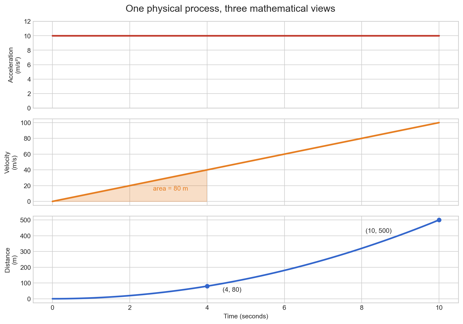
To keep the arithmetic transparent, let us use the approximation \(a=10\ \mathrm{m/s^2}\). Ignore air resistance and suppose the stone begins from rest. Its velocity after \(t\) seconds is
Figure 1: Constant acceleration accumulates into linear velocity, which accumulates into quadratic displacement. The shaded area under the velocity curve through 4 seconds equals 80 m.
Differentiation goes in the reverse direction
Integration answers, “How much change accumulated?” Differentiation asks, “At what rate is this quantity changing now?” The slope of the tangent to the position curve is velocity:
\[
v(t) = \frac{dy}{dt}
\]
The slope of the velocity curve is acceleration:
\[
a(t) = \frac{dv}{dt} = \frac{d^2y}{dt^2}
\]
The fundamental theorem of calculus connects these operations. Under appropriate regularity conditions, differentiation and integration undo one another:
flowchart LR
A["Acceleration a(t)"] -->|integrate| V["Velocity v(t)"]
V -->|integrate| P["Position y(t)"]
P -->|differentiate| V
V -->|differentiate| A
This supplies a language that returns at the end of the module. A population, an inventory, the number of infected people, or the amount of carbon in the atmosphere is a stock. Births, shipments, infections, and emissions are flows. The same mathematics that moves from velocity to position also moves from a social flow to an accumulated social condition.
TipModeling habit: check the units
Acceleration has units \(\mathrm{m/s^2}\). Multiplying or integrating with respect to seconds produces \(\mathrm{m/s}\); integrating again produces meters. Dimensional analysis catches many modeling errors before any computation is performed.
Determinism is not the same as predictability
A model is deterministic when its present state and evolution rule uniquely determine its later state. In the free-fall example, initial position and velocity plus the force law determine the trajectory. This picture inspired an extraordinarily powerful scientific ideal: explain a phenomenon by discovering the state variables and laws that generate it.
Newton also stated four “Rules of Reasoning in Philosophy.” In modern language, they recommend parsimony, consistency of causal explanation, cautious generalization from experiments, and willingness to revise a well-supported proposition when new phenomena require refinement. These are not mechanical instructions for discovery, but they capture a recognizable scientific attitude: use evidence to build general explanations, and hold those explanations provisionally. ### From two bodies to many
The gravitational two-body problem has closed-form orbital solutions: under the standard assumptions, bound orbits are ellipses. Once several bodies interact, however, there is generally no equally simple formula for every trajectory. Numerical approximation remains possible, but some deterministic systems are also chaotic.
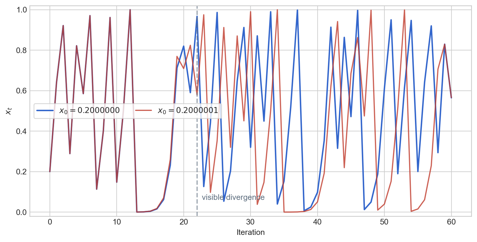
Chaos means that nearby initial states can separate rapidly. It does not mean that the evolution rule contains randomness. To make the distinction visible, consider the logistic map
\[
x_{t+1}=r x_t(1-x_t).
\]
At \(r=4\), two initial values differing by only \(10^{-7}\) eventually produce visibly different paths.
Figure 2: Sensitivity to initial conditions in the deterministic logistic map. The rules are identical and contain no random term, yet finite-precision initial states eventually yield different predictions.
Laplace pushed the deterministic ideal to its philosophical limit. His famous thought experiment imagines an intellect that knows every force and position and possesses enough analytical power to calculate the entire past and future. The idea is now called Laplace’s demon. But the demon silently assumes exact initial conditions, correct and complete laws, a closed system, and effectively unlimited computation. Real inquiry has none of these guarantees. Measurement has finite precision; models omit variables; computation is bounded; and chaotic dynamics amplify small errors. Determinism, therefore, is a claim about the model’s rule, while predictability is a practical relationship among the rule, data, time horizon, and required precision (Hoefer, 2023).
WarningA mistake to avoid
Do not use deterministic as a synonym for easy to predict, and do not use chaotic as a synonym for random. A system can be deterministic, chaotic, and practically unpredictable at the same time.
Check your understanding
Why is velocity linear but displacement quadratic under constant acceleration?
What additional information besides the equations would Laplace’s demon need?
If two simulated paths diverge, what evidence would distinguish deterministic chaos from stochastic noise?
Part II — Statistical laws
Thermodynamics: predictable aggregates from variable particles
Newtonian mechanics focuses attention on individual trajectories. Thermodynamics shows that another kind of scientific description is possible. A gas contains an immense number of molecules with different positions and velocities, yet a small number of macroscopic variables—temperature, pressure, volume, and entropy—can describe it remarkably well.
Sadi Carnot’s 1824 analysis of heat engines asked how efficiently heat could be converted into work. Its lasting lesson is a limit: no cyclic heat engine can convert all absorbed heat into useful work. Later thermodynamics expressed this limitation through the second law.
Temperature is an aggregate
For a monatomic ideal gas, absolute temperature is related to mean translational kinetic energy:
\[
\left\langle \frac12 m v^2 \right\rangle=\frac32 k_B T.
\]
The equation refers to an average. Molecules at the same macroscopic temperature do not all travel at one speed. Their speeds follow a Maxwell–Boltzmann distribution in the idealized classical-gas setting. This matters because a bell-shaped picture should not automatically be labeled “normal”; the speed distribution is asymmetric and restricted to nonnegative values (OpenStax, 2022a).
The conceptual shift is more important than the particular formula:
Show code
flowchart TBM["Microscopic state: many positions and velocities"] --> A["Aggregate description"]A --> T["Temperature"]A --> P["Pressure"]A --> S["Entropy"]
flowchart TB
M["Microscopic state: many positions and velocities"] --> A["Aggregate description"]
A --> T["Temperature"]
A --> P["Pressure"]
A --> S["Entropy"]
We may be unable—or have no need—to track each molecule. Aggregate regularity can exist without identical microscopic behavior. This micro-to-macro reasoning prepares us for population statistics.
Entropy and irreversibility
Classical mechanical equations are often time-reversal symmetric: reverse every velocity in an idealized collision and the reversed motion still satisfies the equations. Macroscopic thermal processes nevertheless have a direction. Heat spontaneously flows from hotter to colder regions; a separated hot and cold gas mixes; coffee approaches room temperature. We do not ordinarily observe the mixed gas spontaneously separating into its original hot and cold halves.
Entropy gives a precise way to discuss this direction. In statistical mechanics,
\[
S=k_B\ln \Omega,
\]
where \(\Omega\) is the number of microscopic configurations compatible with a macrostate. In thermodynamics, a reversible heat transfer satisfies \(dS=\delta Q_{\mathrm{rev}}/T\). “Disorder” can be a useful intuition, but it is not a complete definition. A safer interpretation is that high-entropy macrostates correspond to vastly more compatible microstates and that energy becomes more dispersed and less available to produce organized work (OpenStax, 2022b).
Suppose a box begins with hot gas on the left and cold gas on the right. Removing the partition allows energy exchange. The common-temperature macrostate is overwhelmingly more probable because many more molecular arrangements realize it. Microscopic reversibility is therefore compatible with macroscopic irreversibility. ### Equilibrium and the bathtub equation
A system is in equilibrium when there is no net tendency to change in the absence of an external disturbance. A cup of coffee at room temperature is in thermal equilibrium with the room. A ball at the bottom of a bowl is in a stable mechanical equilibrium.
Equilibrium need not imply inactivity. In a dynamic equilibrium, opposing processes continue but balance. Let \(S(t)\) be the amount of water in a bathtub:
\[
\frac{dS}{dt}=I(t)-O(t),
\]
where \(I(t)\) and \(O(t)\) are inflow and outflow. If \(I=O\), the water level is constant even though water continues to move.
flowchart LR
I["Inflow I(t)"] --> B["Stock S(t)"]
B --> O["Outflow O(t)"]
When decomposition works—and when it does not
Scientific models often divide a system into manageable parts. A Sun–planet pair can sometimes be approximated while neglecting weaker gravitational effects. A chamber can be divided while a barrier prevents exchange. A demographic total can sometimes be approximated by adding independent individual contributions.
Herbert Simon called systems with strong internal interactions and weaker or slower interactions between subsystems nearly decomposable (Simon, 1962). Decomposition is not simply true or false; it is an approximation whose adequacy depends on the question and time scale. It fails when cross-boundary interactions, networks, adaptation, or feedback dominate the phenomenon.
NoteBridge to social science
A citywide unemployment rate is an aggregate property, like temperature, but people are not molecules. They interpret conditions, respond to institutions, form networks, and change the system being measured. Statistical regularity does not justify importing every physical assumption into social analysis.
Comte and the ambition of positive social science
Auguste Comte wrote his six-volume Course of Positive Philosophy between 1830 and 1842. In a Europe transformed by revolution and industrialization, he sought a science that could understand social order and change. He initially called the project social physics and later sociology (Bourdeau, 2026). ### The three stages
Comte proposed that human explanation develops through three stages:
Theological: phenomena are attributed to supernatural will.
Metaphysical: phenomena are explained by abstract entities or essences.
Positive: inquiry gives up the search for absolute causes and instead seeks stable relations among observable phenomena.
Positive philosophy restricts claims to observation and disciplined inference. Scientific progress occurs as increasingly general laws connect broader classes of facts. Comte’s goal was not merely a method for one discipline; it was a unified ordering of knowledge.
A hierarchy of sciences
Comte arranged the sciences from the most general and least complex to the least general and most complex:
flowchart BT
M["Mathematics"] --> A["Astronomy"]
A --> P["Physics"]
P --> C["Chemistry"]
C --> B["Biology"]
B --> S["Sociology"]
On this view, later sciences depend on earlier ones while confronting increasingly complex phenomena. Sociology becomes the final science because social life is the most complicated object of inquiry. Modern research is less comfortably represented by a single ladder. Climate science links physics, chemistry, ecology, economics, politics, and computation in multiple directions. Neuroscience affects psychology while behavior and social environment also alter brains. A network may therefore be a better picture than a strict hierarchy.
Comte’s project remains important because it states an enduring aspiration: social knowledge should be empirical, cumulative, and open to correction. Yet its limitations are equally instructive. Observation is shaped by concepts and institutions. A regularity does not by itself explain a mechanism. Describing what is does not determine what ought to be. People may also change their behavior after learning about a model or policy. Treating society exactly like a celestial body can hide agency, power, meaning, and reflexivity.
Quetelet: from individual uncertainty to population regularity
Adolphe Quetelet brought probability and administrative data into the study of human populations. He examined births, deaths, marriage, height, and recorded crime, arguing that large populations display regularities even though individual biographies remain uncertain. His work helped establish a new meaning of law: not an exact trajectory for each person, but a stable distribution or rate across a population (Jahoda, 2015).
The law of large numbers
Let \(X_1,\ldots,X_n\) be independent and identically distributed random variables with finite mean \(\mu\). The sample mean is
\[
\bar X_n=\frac1n\sum_{i=1}^n X_i.
\]
The weak law of large numbers states that for every \(\varepsilon>0\),
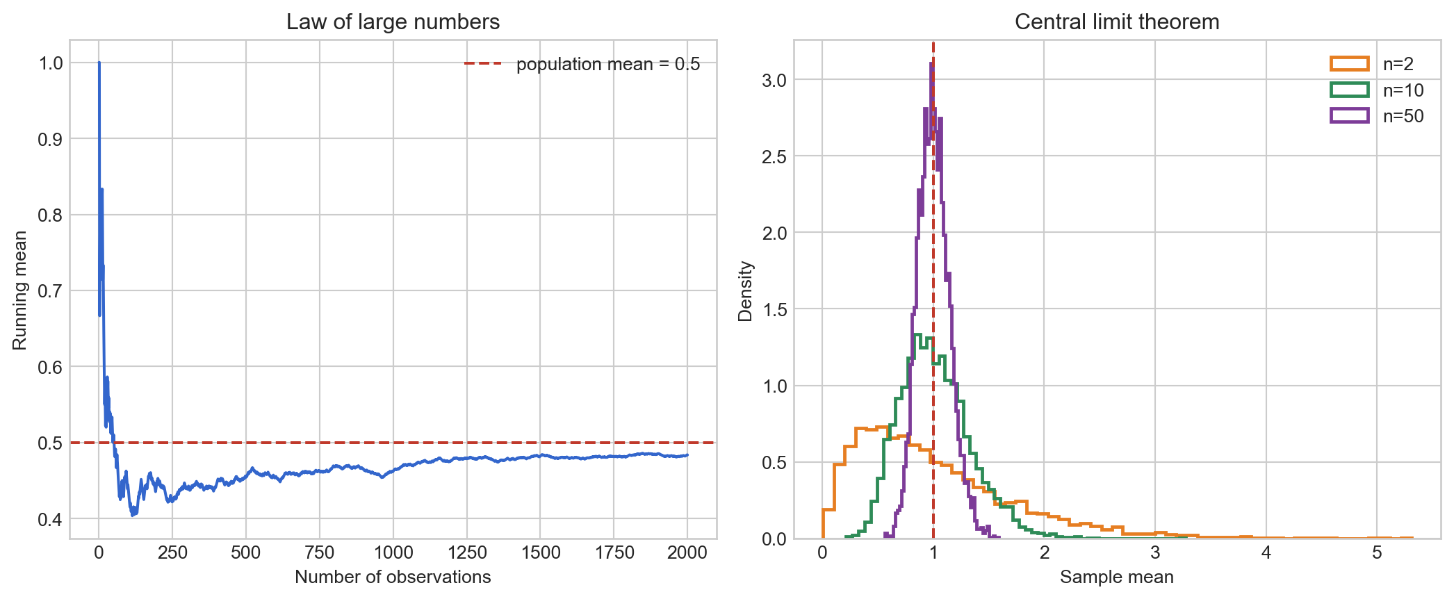
The sample mean stabilizes near the population mean as the sample grows. The law does not say that a short run must look representative, that every population is stable, or that biased data become trustworthy merely because the dataset is large. Dependence, nonstationarity, selection bias, and heavy-tailed distributions can all complicate the conclusion.
Show code
rng = np.random.default_rng(201)n_total =2000draws = rng.binomial(1, 0.5, n_total)running = np.cumsum(draws) / np.arange(1, n_total +1)fig, axes = plt.subplots(1, 2, figsize=(11, 4.6))axes[0].plot(np.arange(1, n_total +1), running, color=COLORS["blue"], lw=1.5)axes[0].axhline(.5, color=COLORS["red"], ls="--", label="population mean = 0.5")axes[0].set(xlabel="Number of observations", ylabel="Running mean", title="Law of large numbers")axes[0].legend()for n, color in [(2, COLORS["orange"]), (10, COLORS["green"]), (50, COLORS["purple"])]: sample_means = rng.exponential(scale=1, size=(6000, n)).mean(axis=1) axes[1].hist(sample_means, bins=55, density=True, histtype="step", lw=1.8, label=f"n={n}", color=color)axes[1].axvline(1, color=COLORS["red"], ls="--")axes[1].set(xlabel="Sample mean", ylabel="Density", title="Central limit theorem")axes[1].legend()fig.tight_layout()plt.show()
Figure 3: Two different limit ideas. Left: one running mean stabilizes near the population mean (LLN). Right: the distribution of many sample means becomes approximately normal and narrows as n grows (CLT).
Do not confuse the LLN with the CLT
The law of large numbers concerns where one sample mean goes as \(n\) grows. The central limit theorem concerns the shape of the sampling distribution across repeated samples. Under common conditions,
The original observations need not be normally distributed. The theorem explains why averages and sums often have approximately normal sampling distributions. It does not say that every dataset becomes normal as its size increases (OpenStax, 2023).
The mean \(\mu\) controls location and the standard deviation \(\sigma\) controls spread. Symmetry makes the mean, median, and mode coincide. Within an appropriately defined population, height and measurement errors may be approximately normal. But income, wealth, city size, network degree, waiting time, and many other social variables are skewed or heavy-tailed. Normality is a model to assess, not a default truth.
L’homme moyen: the “average person”
Quetelet used l’homme moyen—the average person—as an abstraction for studying society. The idea resembles a center of gravity: it need not describe any particular body to summarize a system. This shifted attention from the individual as the only unit of analysis toward properties of populations.
That move was scientifically productive but politically dangerous when the mean was mistaken for an ideal. An average person may not exist, and designing a building, algorithm, medical threshold, or public service for the average can exclude the actual people in the tails. Variation is not noise to be erased; it may be the phenomenon that matters.
Philip Anderson later summarized emergence with the phrase “more is different”: higher levels of organization can exhibit regularities that are not apparent from isolated components (Anderson, 1972). Aggregate description therefore requires new concepts, but it must not erase the mechanisms and inequalities beneath the aggregate.
Recorded crime is a measurement, not a transparent window
Quetelet observed year-to-year regularities in recorded crime and related rates to age, sex, season, place, and social conditions. This challenged explanations based only on individual morality and suggested prevention, education, and institutional reform as possible policy levers.
Modern data science must add a crucial measurement warning. Recorded crime is jointly produced by underlying behavior and by law, reporting, surveillance, police deployment, classification, and administrative practice. A rise in a crime dataset may reflect increased offending, increased reporting, changed definitions, intensified enforcement, or some combination. Population association also does not establish an individual causal mechanism. The data-generating institution belongs inside the model.
ImportantThree levels that must remain distinct
Individual claim: what a particular person will do.
Population claim: how a rate or distribution behaves across many people.
Institutional measurement claim: how a social process becomes a recorded variable.
An analysis can be correct at one level and wrong at another.
Part III — Causal laws and scientific uncertainty
Fisher: measurement error becomes part of the model
R. A. Fisher’s Statistical Methods for Research Workers (1925) and The Design of Experiments (1935) helped formalize a statistical approach to scientific uncertainty. The point is not that science should accept careless measurement. It is that variability cannot simply be wished away. Measurement, sampling, biological heterogeneity, and experimental conditions all generate variation. Scientific inference must describe that variation.
Accuracy, precision, and bias
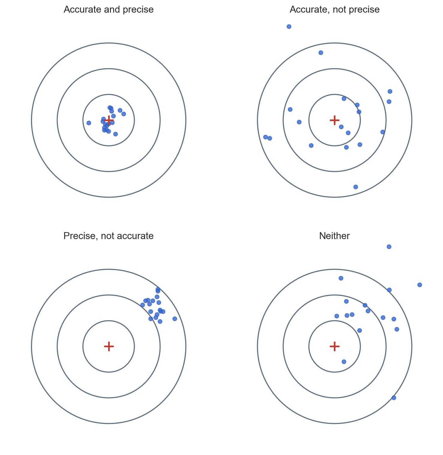
Accuracy is closeness to the target or true value. Precision is repeatability: how tightly repeated measurements cluster. A procedure may be precise but inaccurate when systematic error moves every result away from the target.
For an estimator \(\hat\theta\) of a parameter \(\theta\), statistical bias is
Bias is a long-run property of the procedure, not a synonym for one estimate being wrong. Nor is it identical to social or algorithmic unfairness, though measurement and sampling biases can contribute to unfair systems.
Replication supplies information about this variability. Repeated measurements assess repeatability; repeated experimental units help estimate experimental variation; independent replication of an entire study tests whether a finding survives changes of investigator, location, or time. These are related but not interchangeable.
Randomization and causal inference
An association between fertilizer and pumpkin weight does not by itself tell us that the fertilizer caused heavier pumpkins. Perhaps the new fertilizer was applied to sunnier plots, healthier plants, or a different soil type. These variables are confounders: they influence treatment assignment, outcome, or both.
The causal question is counterfactual. For pumpkin \(i\), let
\[
Y_i(1)=\text{weight under the new fertilizer},\qquad
Y_i(0)=\text{weight under the old fertilizer}.
\]
The individual treatment effect is \(Y_i(1)-Y_i(0)\), but only one potential outcome can be observed for the same pumpkin. Random assignment does not solve this missing-data problem at the individual level. It makes treatment groups comparable in expectation, permitting estimation of an average treatment effect: \[
\widehat{\tau}=\bar Y_{\text{new}}-\bar Y_{\text{old}}.
\] ### Four principles of experimental design
Control: create a meaningful comparison condition.
Randomize: assign treatments by chance to break systematic links between treatment and background variables.
Replicate: apply each treatment to multiple independent experimental units.
Block: group similar units by important nuisance variables, then randomize within blocks.
Blocking is useful when a known nuisance factor—such as field location, batch, operator, or time of day—could obscure the treatment contrast. It reduces unwanted variability without making the nuisance factor the scientific focus (NIST/SEMATECH, 2012).
Worked design: the pumpkin fertilizer experiment
Suppose we have 40 pumpkin plants across four garden rows. Soil moisture differs by row.
Experimental unit: one independently treated pumpkin plant.
Treatment: new versus old fertilizer.
Block: garden row.
Assignment: within each row, randomly assign half the plants to each fertilizer.
Outcome: pre-specified fruit weight at harvest.
Estimand: average difference in weight caused by assignment to the new fertilizer for these experimental conditions.
Analysis: compare group means using the randomization distribution generated by treatment reassignments that respect the blocks.
Randomization addresses internal validity for the assigned experiment. It does not automatically establish that the result generalizes to another pumpkin variety, climate, dose, or year. Causal identification and external validity are different problems.
The Lady Tasting Tea and the logic of a p-value
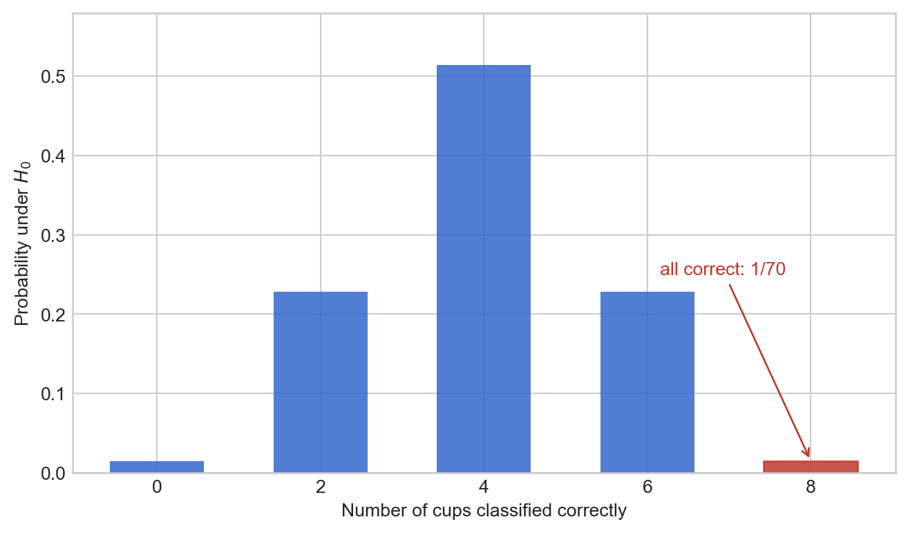
Fisher’s famous example begins with a claim: a woman says she can tell whether milk or tea was poured first. In the exact design, eight cups are prepared—four by each method—and the taster is told that there are four of each. She must select the four cups prepared by one method (Fisher, 1935).
Under the null hypothesis that she cannot discriminate and is effectively guessing among allowed allocations, there are
\[
{8\choose4}=70
\]
equally possible selections. Only one selection gets all four cups correct, so
\[
P(\text{all four correct}\mid H_0)=\frac1{70}\approx0.0143.
\]
This is not the same as four or five independent 50/50 guesses. For example, five independent correct guesses would have probability
\[
\left(\frac12\right)^5=0.03125,
\]
Show code
# If j of the four milk-first cups are selected correctly, then 2j cups are# classified correctly overall. Count selections with C(4,j)C(4,4-j).j = np.arange(5)correct_total =2* jprob = np.array([math.comb(4, int(k)) * math.comb(4, 4-int(k)) for k in j]) / math.comb(8, 4)fig, ax = plt.subplots(figsize=(8, 4.5))bars = ax.bar(correct_total, prob, width=1.15, color=COLORS["blue"], alpha=.85)bars[-1].set_color(COLORS["red"])ax.annotate("all correct: 1/70", xy=(8, prob[-1]), xytext=(6.15, .25), arrowprops={"arrowstyle": "->", "color": COLORS["red"]}, color=COLORS["red"])ax.set(xlabel="Number of cups classified correctly", ylabel="Probability under $H_0$", xticks=correct_total, ylim=(0, .58))plt.show()
Figure 5: The exact null distribution for Fisher’s eight-cup design. If the taster selects four cups, the probability of exactly k correct identifications follows a finite combinatorial distribution.
A p-value is the probability, calculated under the null model, of obtaining a test statistic at least as extreme as the observed one:
\[
p=P(T\ge T_{\mathrm{obs}}\mid H_0),
\]
with the direction and definition of “extreme” chosen by the test. It is not\(P(H_0\mid\text{data})\). It is also not the probability that the result occurred “by chance,” the probability that replication will fail, or a measure of effect size. The American Statistical Association emphasizes that scientific conclusions should not be based only on whether a p-value crosses a threshold; study design, effect magnitude, uncertainty, prior evidence, and consequences all matter (Wasserstein & Lazar, 2016).
NoteStatistical significance is not practical importance
With a very large sample, a tiny and practically irrelevant effect can yield a small p-value. With a small noisy sample, an important effect may remain uncertain. Report the estimated effect and its uncertainty, and ask whether the magnitude matters in context.
Limits of experiments
Randomized experiments are powerful but not universal. Some interventions are unethical, too expensive, too slow, impossible to enforce, or affected by interference between units. Social experiments may change behavior simply because participants know they are being studied. Results can also be local to a population, institution, and historical moment. When randomization is unavailable, researchers use natural experiments, quasi-experimental designs, structural models, and carefully justified observational assumptions—but no method makes design questions disappear.
Part IV — Systemic laws
Georgescu-Roegen: the economy is not a closed circular diagram
Standard economic diagrams often show a circular flow: households supply labor, firms produce goods, income returns to households, and expenditure returns to firms. Nicholas Georgescu-Roegen argued that this monetary circulation leaves out the physical throughput that makes economic activity possible. Production takes concentrated, useful matter and energy from the environment and returns lower-quality energy, dispersed materials, and waste (Georgescu-Roegen, 1971, 1975).
Show code
flowchart LRR["Concentrated resources"] --> P["Production and consumption"]P --> G["Goods and services"]P --> W["Dispersed energy and waste"]
flowchart LR
R["Concentrated resources"] --> P["Production and consumption"]
P --> G["Goods and services"]
P --> W["Dispersed energy and waste"]
He distinguished available or “free” energy—energy gradients that humans can use—from bound energy, such as diffuse ambient heat that cannot readily perform useful work. The economic process is therefore not perfectly reversible. Recycling can reduce new extraction and waste, but recycling itself requires energy and cannot recover every dispersed material without loss.
The boundary of the claim matters. Earth is not energetically closed: it continually receives low-entropy solar radiation and emits energy to space. It is much closer to materially closed on human time scales. Local systems can become more ordered by exporting entropy to their surroundings. Living organisms do this constantly. The second law does not say that local growth or organization is impossible; it says that the full physical accounting must include the environment and the irreversibility of transformation.
Georgescu-Roegen’s contribution is best understood as a boundary correction. An economic model that tracks only money can be internally consistent yet omit the material conditions on which the modeled economy depends. Every computational model similarly draws a boundary. What crosses that boundary as an unexplained “external input” may determine whether its conclusions remain credible.
Forrester and system dynamics
Jay W. Forrester developed system dynamics to study systems whose behavior arises from feedback, accumulation, nonlinear relationships, and delay. A computer simulation makes assumptions explicit enough to execute consistently and inspect. This is valuable because informal mental models often omit feedback or apply incompatible assumptions at different points. But executability is not truth: a precisely coded model can still have the wrong boundary, equations, parameters, or interpretation (Forrester, 1971).
Stocks and flows return
For any stock \(S(t)\),
\[
S(t)=S(0)+\int_0^t[I(u)-O(u)]\,du,
\]
or equivalently,
\[
\frac{dS}{dt}=I(t)-O(t).
\]
This is the free-fall calculus in a new domain. The stock remembers the history of net flows. If weekly orders suddenly fall to zero, inventory does not necessarily become zero; its level depends on everything received and shipped before that moment.
Domain
Stock
Inflow
Outflow
Population
People living in a city
Births and in-migration
Deaths and out-migration
Public health
Currently infected people
New infections
Recoveries and deaths
Supply chain
Inventory
Deliveries
Shipments
Environment
Atmospheric carbon
Emissions
Natural and engineered removal
Education
Enrolled students
Admissions
Graduation and withdrawal
Feedback loops
A reinforcing loop amplifies change. More adopters generate more word of mouth, which produces still more adopters. A balancing loop opposes change. Low inventory triggers more ordering, which eventually rebuilds inventory. The sign describes the loop’s direction, not whether it is morally good or bad.
Show code
flowchart LRA["Adopters"] -->|+| W["Word of mouth"]W -->|+| A
flowchart LR
A["Adopters"] -->|+| W["Word of mouth"]
W -->|+| A
flowchart LR
I["Inventory"] -->|−| G["Inventory gap"]
G -->|+| O["Orders"]
O -->|after delay, +| I
The second loop seeks balance, yet the delay can make it oscillate. Decision-makers see a shortage and order more. Before those orders arrive, they see the shortage again and order still more. When the delayed shipments finally arrive, inventory overshoots. The same correction mechanism then operates in reverse.
Policy resistance
Forrester used simulation to argue that plausible policies can generate results opposite to those intended. Suppressing every small fire may allow fuel to accumulate, increasing the potential severity of later fires. Adding road capacity can lower travel time initially, encourage additional trips or relocation, and recreate congestion. These examples do not prove that suppression or road expansion is always wrong. They show why an immediate local effect is not the same as a long-run system effect. Boundaries, adaptation, feedback, and delay must be modeled.
The Beer Game: reasonable people, unstable system
The Beer Distribution Game represents a supply chain with a retailer, wholesaler, distributor, and factory. Each stage receives customer orders, ships from inventory, and places replenishment orders upstream. Information and deliveries take time. Each participant sees only a local part of the chain.
flowchart RL

C["Customers"] -->|orders| R["Retailer"]
R -->|orders| W["Wholesaler"]
W -->|orders| D["Distributor"]
D -->|orders| F["Factory"]
F -.->|delayed shipments| D
D -.->|delayed shipments| W
W -.->|delayed shipments| R
R -.->|sales| C
A modest and permanent increase in customer demand can produce larger oscillations upstream. Participants attempt to correct shortages, but they do not fully account for orders already in the pipeline. The resulting bullwhip effect is emergent: the collective instability is not a direct copy of customer demand and need not be intended by any participant. Experiments with the game show that the interaction between human decision rules and the system’s delayed feedback structure produces aggregate behavior far from the stable optimum (Sterman, 1989).
The lesson is not simply “people are irrational.” Even a sensible local rule can perform badly inside a system whose state is only partly visible. Better decisions may require shared information, explicit accounting for the supply line, redesigned incentives, shorter delays, or structural changes—not merely telling each participant to try harder.
TipHow to read a system-dynamics model
Ask five questions:
What are the stocks?
Which flows change each stock?
Which feedback loops connect decisions to later conditions?
Where are the delays?
What important process lies outside the model boundary?
Synthesis — four meanings of scientific explanation
The module began with a stone and ended with a supply chain. The path is coherent because each stage expands what counts as a scientifically intelligible pattern.
Worldview
Central object
Meaning of a law
Main tool
Characteristic limitation
Newtonian mechanics
State and trajectory
Exact evolution rule
Differential equations
Chaos, finite measurement, and incomplete models
Statistical social science
Population and distribution
Stable aggregate regularity
Probability and statistics
Aggregation may hide mechanisms, change, or measurement bias
Fisherian experiment
Treatment contrast
Causal effect under an assignment design
Randomization and inference
Ethical, practical, interference, and generalization limits
System dynamics
Stocks, flows, feedback, and delay
Endogenous pattern generated by structure
Simulation
Conclusions depend on boundaries and assumptions
Show code
flowchart TBQ["What must the explanation recover?"]Q --> T["Trajectory → deterministic model"]Q --> R["Regularity → statistical model"]Q --> C["Intervention effect → causal design"]Q --> S["Emergent behavior → systems model"]
Calculus explains accumulation and instantaneous change. Probability explains stable patterns amid individual variation. Experimental design separates intervention effects from background differences under a defined assignment process. System dynamics explains how local decisions, feedback, and delay generate collective behavior.
Computational social science needs all four, but it should not confuse their claims. A predictive association is not automatically causal. A population regularity does not determine an individual’s future. A causal estimate from one experiment is not a universal law. A simulation does not become evidence merely because it runs. The scientist’s task is to connect the kind of question, the model, the data-generating process, and the strength of the conclusion.
A final diagnostic
When a social model fails, ask which failure occurred:
State failure: important variables or initial conditions were missing.
Stochastic failure: variability or dependence was modeled incorrectly.
Measurement failure: the recorded variable did not faithfully represent the intended concept.
Causal failure: treatment assignment or confounding did not support the claimed intervention effect.
Boundary failure: an “external” process actually drove the result.
Feedback failure: adaptation, accumulation, or delay was omitted.
Scale failure: a relationship at one level was incorrectly transferred to another.
There is no single universal fix called “more data.” Sometimes we need better measurement, a different design, a new state variable, a longer time horizon, a revised boundary, or an entirely different form of explanation.
Schuler, J. S. (2026). Module I: Mathematical, physical, and social foundations [Course slides]. Department of Computational and Data Sciences, George Mason University.
Simon, H. A. (1962). The architecture of complexity. Proceedings of the American Philosophical Society, 106(6), 467–482.