Data Modeling - Clustering

Clustering is the unsupervised task of organizing observations into groups so that observations assigned to the same group are similar according to some criterion, while observations in different groups are comparatively dissimilar. Unlike supervised learning, clustering begins without a target variable that identifies the desired partition.

Let \(\mathcal D=\{x_1,x_2,\ldots,x_N\}, x_n\in\mathcal X\), be an unlabeled dataset. A hard clustering into \(K\) groups is a collection \(\mathcal C=\{C_1,\ldots,C_K\}\) satisfying

\[ C_k\subseteq \{1,\ldots,N\},\qquad C_k\cap C_\ell=\varnothing \text{ for }k\neq \ell, \] and \[ \bigcup_{k=1}^{K}C_k=\{1,\ldots,N\}. \]

Equivalently, clustering assigns each observation a latent label \(z_n\in\{1,\ldots,K\}\).

However, this formal definition does not determine what a cluster is. Different algorithms embody different concepts of grouping:

Therefore, clustering is not one uniquely defined mathematical problem. It is a collection of unsupervised methods based on different structural assumptions. It asks:

What form of structure would constitute a meaningful cluster in this dataset?

1. Data Geometry Before Clustering

1.1. Representation Determines the Clusters

A clustering algorithm operates on a representation of the observations. Suppose an observation is represented as \(x_n=(x_{n1},\ldots,x_{nD})^\top\in\mathbb R^D\).

Even before selecting an algorithm, the analyst has made consequential choices:

  • which variables define similarity;
  • whether variables are transformed;
  • how missingness is handled;
  • whether observations are aggregated;
  • whether time, geography, or network structure is included;
  • whether raw variables or learned embeddings are used.

Two observations can be near each other in one representation and far apart in another. Thus, clustering does not reveal structure independently of representation. It reveals structure under a specified geometry or probability model.

1.2. Distances and Dissimilarities

Many clustering methods begin with a distance or dissimilarity function \(d:\mathcal X\times\mathcal X\rightarrow[0,\infty).\) For numerical vectors, common choices include the Euclidean distance

\[ d_2(x_i,x_j) = \left[ \sum_{r=1}^{D}(x_{ir}-x_{jr})^2 \right]^{1/2}, \]

Manhattan distance

\[ d_1(x_i,x_j) = \sum_{r=1}^{D}|x_{ir}-x_{jr}|, \]

and Mahalanobis distance

\[ d_M(x_i,x_j) = \sqrt{ (x_i-x_j)^\top \Sigma^{-1} (x_i-x_j) }. \]

For binary variables, Hamming or Jaccard dissimilarities may be more appropriate. For text vectors, cosine dissimilarity is often used:

\[ d_{\cos}(x_i,x_j) = 1- \frac{x_i^\top x_j} {\|x_i\|_2\|x_j\|_2}. \]

For mixed numerical and categorical variables, Gower-type dissimilarities combine variable-specific distances.

1.3. Scaling

Suppose customer observations contain: \[ \begin{aligned} x_1 &= \text{annual income in dollars},\\ x_2 &= \text{number of purchases},\\ x_3 &= \text{average review score}. \end{aligned} \]

Under Euclidean distance,

\[ \|x_i-x_j\|_2^2 = (x_{i1}-x_{j1})^2 + (x_{i2}-x_{j2})^2 + (x_{i3}-x_{j3})^2. \]

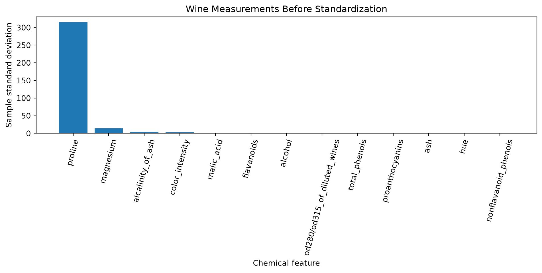
Income may dominate because of its numerical units. Standardization replaces each feature by

\[ z_{nr} = \frac{x_{nr}-\bar x_r}{s_r}. \]

After standardization, the algorithm works in units of marginal standard deviations. Raw-scale clustering asks which observations are close in physical measurement units. Standardized clustering asks which observations have similar relative profiles across variables.

Robust scaling may be preferable when features contain extreme values:

\[ z_{nr}^{\text{robust}} = \frac{x_{nr}-\operatorname{median}(x_r)} {\operatorname{IQR}(x_r)}. \]

1.4. Missing Values

Many clustering implementations require complete numerical matrices. Common responses include:

  • deleting incomplete observations;
  • median or model-based imputation;
  • multiple imputation followed by stability analysis;
  • defining distances using jointly observed variables;
  • using probabilistic models that treat missing values as latent.

If a distance is computed from only jointly observed coordinates,

\[ O_{ij} = \{r:x_{ir}\text{ and }x_{jr}\text{ are observed}\}, \]

an adjusted Euclidean distance may be

\[ d(x_i,x_j) = \sqrt{ \frac{D}{|O_{ij}|} \sum_{r\in O_{ij}} (x_{ir}-x_{jr})^2 }. \]

However, pairwise missingness can cause different distances to be based on different coordinate sets, making the resulting geometry difficult to interpret.

Imputation may create artificial concentration near central values and can therefore generate apparent clusters or remove genuine ones. Missingness indicators and sensitivity analysis are often necessary.

1.5. Outliers and Rare Groups

An extreme observation may be:

  • an error;
  • an isolated anomaly;
  • an early sign of system failure;
  • a member of a small but meaningful cluster;
  • a valid observation from a different population.

The treatment depends on the scientific question. K-means can be strongly influenced by extreme observations because it minimizes squared distances. K-medoids is more resistant. DBSCAN may classify isolated points as noise. A mixture model may create a small component around them.

Calling a point “noise” is itself a modeling judgment. Rare observations are not automatically meaningless.

1.6. Cluster Tendency

Before forcing a partition, one should ask whether the data exhibit clustering tendency at all.

A clustering algorithm can partition almost any dataset, even a uniform cloud. The existence of an output does not prove the existence of meaningful clusters.

Useful questions include:

  • Are there multimodal marginal or projected distributions?
  • Are within-group distances systematically smaller than between-group distances?
  • Is the partition stable across samples, initializations, and feature choices?
  • Does the result outperform structure expected under a reference null distribution?
  • Are the clusters interpretable through variables not used to construct them?
  • Does the cluster solution support a meaningful downstream action?

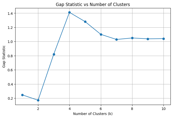
The gap statistic explicitly compares within-cluster dispersion against that expected under a reference distribution with no comparable cluster structure

2. \(k\)-Means Clustering

2.1. The \(k\)-Means Objective

Assume \(x_n\in\mathbb R^D\) and choose a number of clusters \(K\).

Let \(z_{nk}\in\{0,1\}\) indicate whether point \(n\) is assigned to cluster \(k\), with \(\sum_{k=1}^{K}z_{nk}=1.\) Let \(\mu_k\in\mathbb R^D\) be the centroid of cluster \(k\).

The K-means objective is

\[ J(Z,\mu) = \sum_{n=1}^{N} \sum_{k=1}^{K} z_{nk}\|x_n-\mu_k\|_2^2. \] Equivalently, if \(C_k\) is the index set of cluster \(k\),

\[ J(\mathcal C) = \sum_{k=1}^{K} \sum_{n\in C_k} \|x_n-\mu_k\|_2^2. \]

This is called:

  • within-cluster sum of squares;
  • within-cluster dispersion;
  • quantization error;
  • distortion;
  • inertia.

2.2. The Optimal Centroid

NoteTheorem: The Mean Minimizes Squared Distance

For a fixed nonempty cluster C, the point \[ \mu^* = \frac{1}{|C|} \sum_{n\in C}x_n \]

minimizes

\[ J_C(\mu) = \sum_{n\in C}\|x_n-\mu\|_2^2. \]

TipProof

Expand:

\[ J_C(\mu) = \sum_{n\in C} (x_n-\mu)^\top(x_n-\mu). \]

Differentiate with respect to \(\mu\):

\[ \nabla_\mu J_C(\mu) = -2\sum_{n\in C}(x_n-\mu). \]

Setting the gradient equal to zero gives

\[ \sum_{n\in C}x_n-|C|\mu=0. \]

Therefore,

\[ \mu = \frac{1}{|C|} \sum_{n\in C}x_n. \]

The Hessian is \(\nabla_\mu^2J_C(\mu)=2|C|I\), which is positive definite for a nonempty cluster. Hence the stationary point is the unique minimizer.

2.3. Lloyd’s Algorithm

The joint optimization over assignments and centroids is nonconvex. Lloyd’s algorithm alternates between two simpler minimization steps.

Assignment step

For fixed centroids, assign each point to its closest centroid:

\[ z_{nk} = \begin{cases} 1, & k=\displaystyle\arg\min_j \|x_n-\mu_j\|^2,\\[6pt] 0, &\text{otherwise}. \end{cases} \]

Update step

For fixed assignments, set \[ \mu_k = \frac{ \sum_{n=1}^{N}z_{nk}x_n }{ \sum_{n=1}^{N}z_{nk} }. \]

The procedure repeats until assignments stop changing, centroids move less than a tolerance, or the objective improvement becomes negligible.

2.4. Monotonicity and Finite Termination

NoteTheorem 2: Lloyd’s Algorithm Does Not Increase the Objective

Each complete iteration of Lloyd’s algorithm satisfies

\[ J^{(t+1)}\leq J^{(t)}. \]

TipProof

During the assignment step, centroids are fixed. Each point is assigned to the closest centroid, so its squared-distance contribution cannot increase.

Therefore,

\[ J(Z^{(t+1)},\mu^{(t)}) \leq J(Z^{(t)},\mu^{(t)}). \]

During the update step, assignments are fixed. By Theorem 1, replacing each centroid with the mean of its assigned observations minimizes the within-cluster squared error.

Thus,

\[ J(Z^{(t+1)},\mu^{(t+1)}) \leq J(Z^{(t+1)},\mu^{(t)}). \]

Combining both inequalities gives

\[ J^{(t+1)}\leq J^{(t)}. \]

Because only finitely many hard partitions of \(N\) observations into \(K\) labeled groups exist, the algorithm eventually reaches a fixed assignment under ordinary tie-handling conditions. However, the result may be only a local optimum.

2.5. Geometry of \(K\)-Means

The assignment region of centroid \(\mu_k\) is

\[ V_k = \left\{ x: \|x-\mu_k\| \leq \|x-\mu_j\| \text{ for all }j \right\}. \]

These regions form a Voronoi partition. Under Euclidean distance, boundaries between two centroids are hyperplanes.

For centroids \(\mu_a\) and \(\mu_b\), the boundary satisfies

\[ \|x-\mu_a\|^2 = \|x-\mu_b\|^2. \]

Expanding and cancelling \(x^\top x\),

\[ -2x^\top\mu_a+\|\mu_a\|^2 = -2x^\top\mu_b+\|\mu_b\|^2. \]

Therefore, \[ 2x^\top(\mu_b-\mu_a) = \|\mu_b\|^2-\|\mu_a\|^2. \]

Hence the boundary is linear.

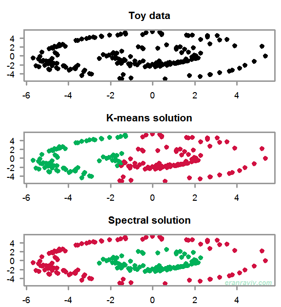
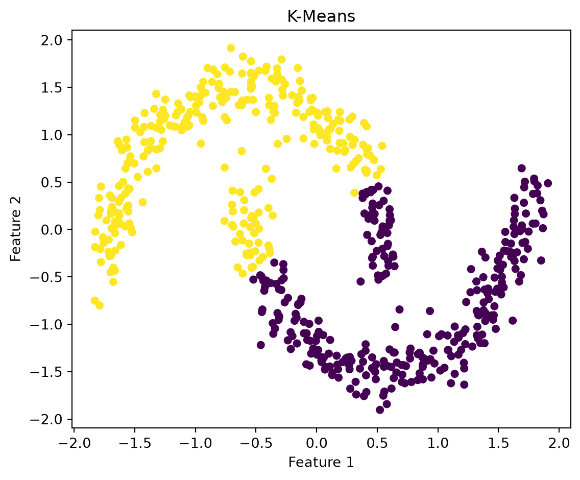
This explains why K-means favors clusters that can be separated by centroid-based Voronoi cells. It is poorly matched to intertwined spirals, rings, highly unequal densities, or strongly nonconvex shapes.

2.6. Bias Toward Spherical, Similar-Scale Clusters

The squared Euclidean objective works best when groups are approximately:

  • compact;
  • convex;
  • spherical or isotropic;
  • similar in spread;
  • sufficiently separated.

Suppose one genuine cluster is large and diffuse while another is small and compact. Reducing squared error may split the diffuse group and merge the compact group with a neighbor. The optimization objective need not recover the grouping a human expects.

K-Means

3. \(k\)-Medoids and Robust Prototypes

In \(K\)-medoids, each cluster center must be an observed object.

Let \(m_k\in\{1,\ldots,N\}\) be the index of medoid \(k\). Then

\[ J_{\text{medoid}} = \sum_{n=1}^{N} \min_{k} d(x_n,x_{m_k}). \]

Because the prototype is an actual observation, \(K\)-medoids can work with an arbitrary dissimilarity matrix and does not require a meaningful coordinate mean.

For a fixed cluster \(C_k\), its medoid is

\[ m_k^* = \arg\min_{j\in C_k} \sum_{i\in C_k} d(x_i,x_j). \]

Advantages include:

  • greater robustness to outliers;
  • compatibility with non-Euclidean distances;
  • interpretable prototypes;
  • support for categorical or structured objects when a dissimilarity is defined.

The main disadvantage is greater computational expense compared with standard \(K\)-means.

K-Medoids

4. Selecting the Number of Clusters

4.1. The Elbow Method

Define

\[ W_K = \sum_{k=1}^{K} \sum_{n\in C_k} \|x_n-\mu_k\|^2. \] Because additional clusters cannot increase the optimal within-cluster error,

\[ W_{K+1}\leq W_K. \]

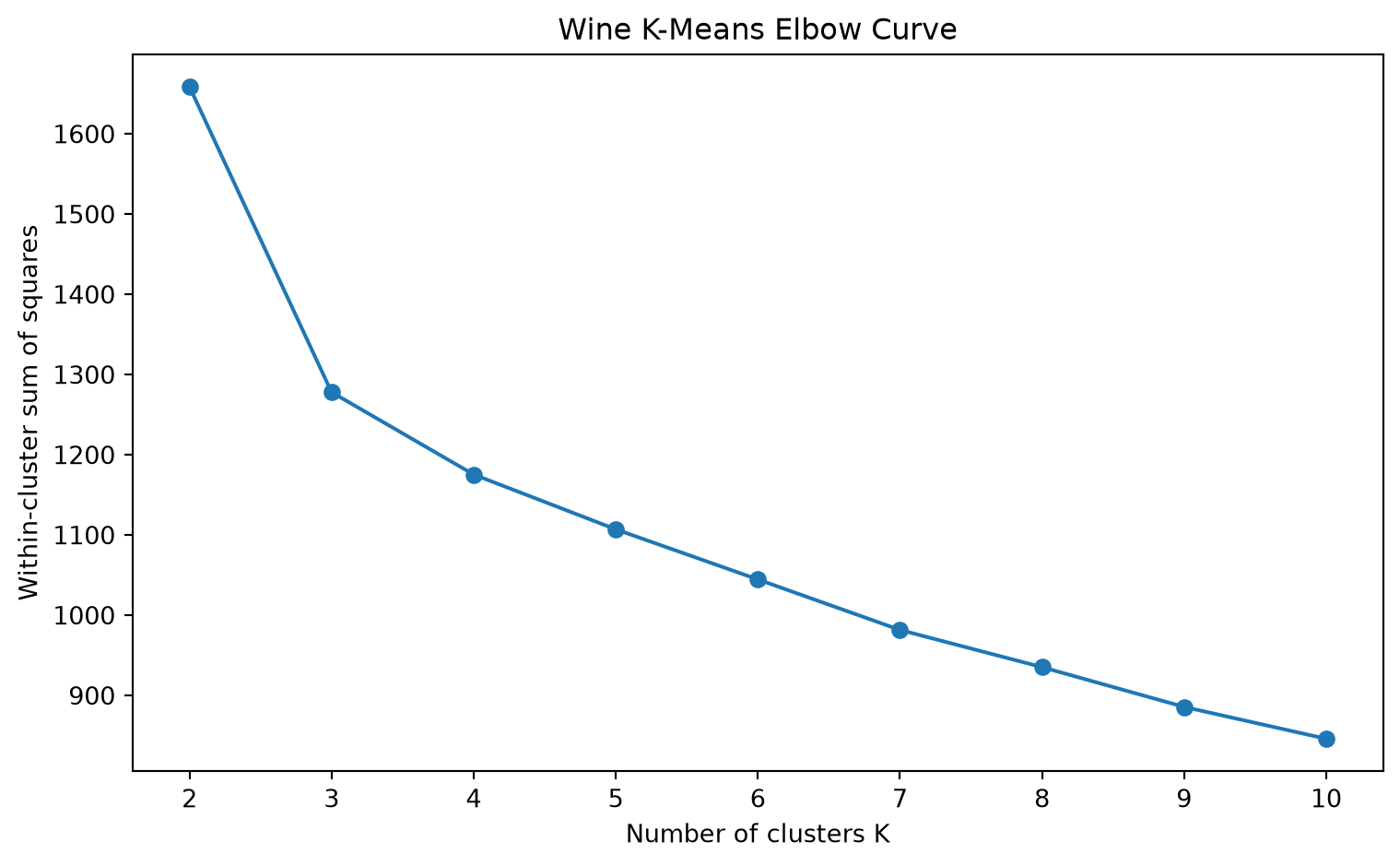
The elbow method plots \(W_K\) against \(K\) and searches for a point after which additional clusters yield comparatively small reductions.

The difficulty is that many datasets have no clear elbow. The method is descriptive, not a theorem establishing the true number of groups.

The Elbow Method

4.2. Silhouette Coefficient

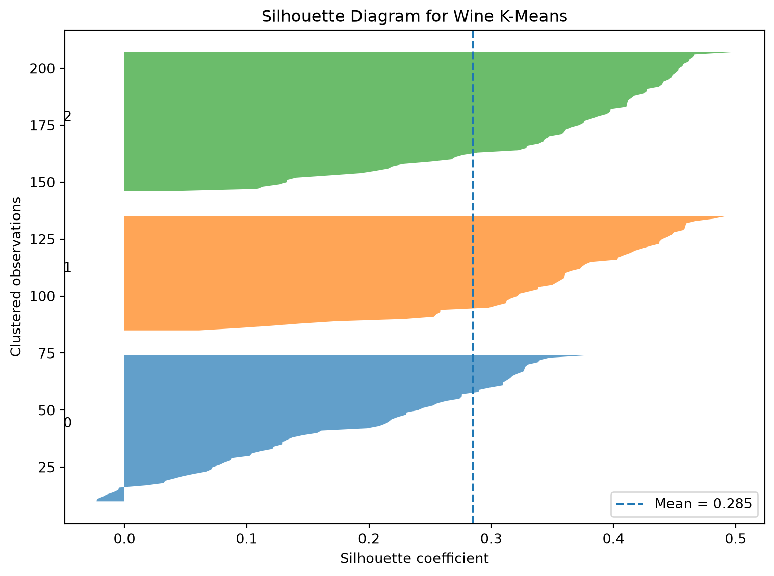
For observation \(i\), let \(a(i)\) be its average dissimilarity to other observations in its assigned cluster.

For each other cluster \(C\), compute the average dissimilarity from i to that cluster. Let

\[ b(i) = \min_{C\neq C(i)} \frac{1}{|C|} \sum_{j\in C}d(x_i,x_j). \]

The silhouette value is

\[ s(i) = \frac{b(i)-a(i)} {\max\{a(i),b(i)\}}. \]

Then \(-1\leq s(i)\leq 1\).

Interpretation:

  • \(s(i)\approx 1\): the point is well matched to its cluster;
  • \(s(i)\approx 0\): it lies near a boundary;
  • \(s(i)<0\): another cluster may fit it better.

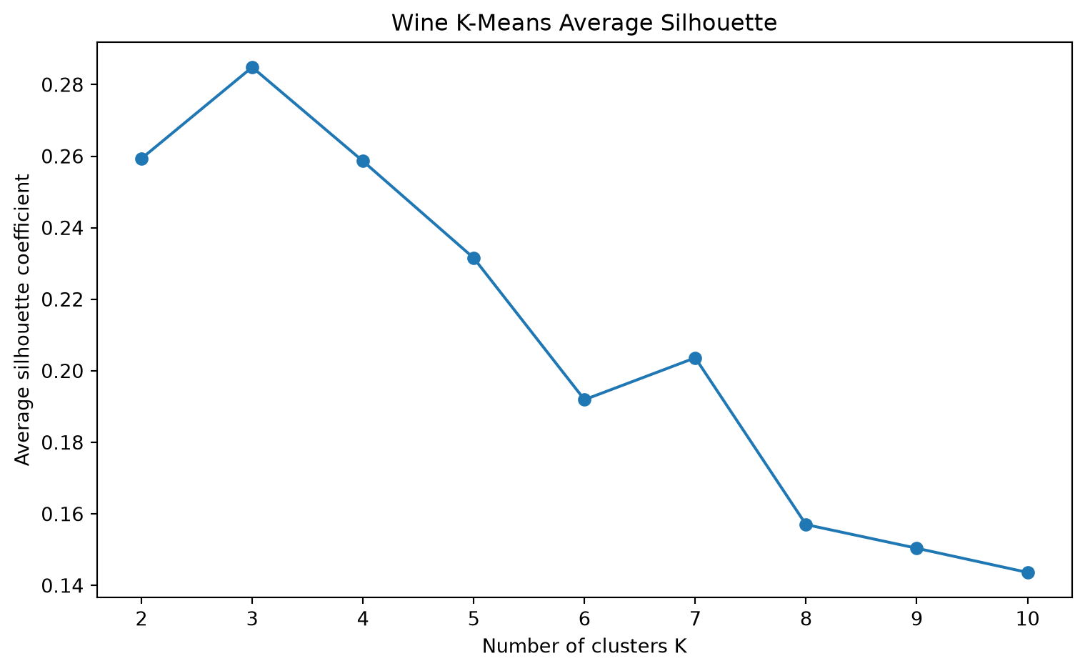
The average silhouette is

\[ \bar s = \frac{1}{N}\sum_{i=1}^{N}s(i). \]

Rousseeuw introduced silhouettes as both a numerical and graphical aid to interpreting partition quality.

Silhouette analysis inherits the chosen distance and tends to favor separated, compact clusters. A high score is not proof of substantive validity.

Silhouette Coefficient

4.3. Gap Statistic

Let W_K be within-cluster dispersion for the observed data. Generate B reference datasets from a null distribution with no comparable cluster structure and calculate

\[ W_{Kb}^*, \qquad b=1,\ldots,B. \]

The gap statistic is

\[ \operatorname{Gap}(K) = \frac{1}{B} \sum_{b=1}^{B} \log W_{Kb}^* - \log W_K. \]

A large gap means the observed clustering achieves substantially lower dispersion than expected under the reference distribution.

Define

\[ s_K = \sqrt{1+\frac{1}{B}} \operatorname{sd} \left( \log W_{K1}^*,\ldots,\log W_{KB}^* \right). \]

A common selection rule chooses the smallest \(K\) satisfying

\[ \operatorname{Gap}(K) \geq \operatorname{Gap}(K+1)-s_{K+1}. \]

The result depends on the reference distribution and feature-space geometry.

Gap Statistic

4.4. Stability-Based Selection

A clustering solution should not change radically because a small fraction of observations was removed.

A stability procedure may:

  1. resample observations;
  2. refit clustering;
  3. match clusters across fits;
  4. compare partitions using an agreement index;
  5. examine how stability changes with \(K\).

Instability may indicate:

  • weak cluster separation;
  • an inappropriate \(K\);
  • high sensitivity to initialization;
  • redundant or noisy features;
  • a continuum rather than discrete groups.

Extreme stability can also arise from a strong nuisance variable, so stability should be interpreted with substantive diagnostics.

5. Hierarchical Clustering

5.1. Nested Partitions

Hierarchical clustering produces a sequence of nested partitions rather than one partition for a prespecified \(K\).

Agglomerative clustering starts with

\[ \mathcal C^{(N)} = \{\{1\},\{2\},\ldots,\{N\}\} \]

and repeatedly merges two clusters until one remains.

Divisive clustering begins with all observations in one group and recursively splits them.

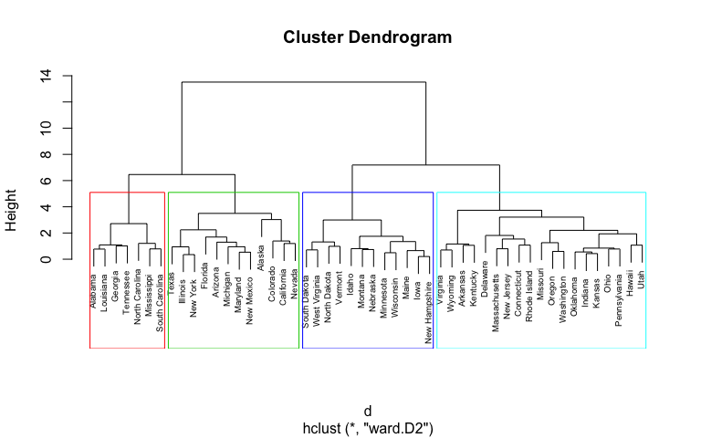
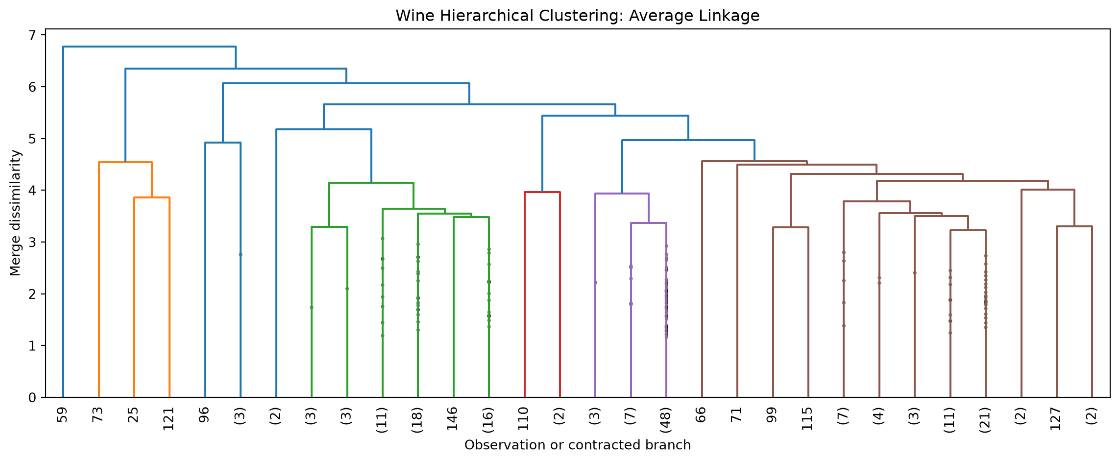
The result is represented by a dendrogram. The vertical merge height records the dissimilarity at which two branches were joined.

5.2. Agglomerative Algorithm

Given pairwise dissimilarities:

  1. Initialize every observation as a singleton cluster.
  2. Compute dissimilarities between all clusters.
  3. Merge the pair with minimum linkage dissimilarity.
  4. Update the cluster dissimilarities.
  5. Repeat until one cluster remains.

The linkage rule defines the meaning of distance between sets.

5.2.1 Single Linkage

For clusters A and B,

\[ d_{\text{single}}(A,B) = \min_{i\in A,j\in B} d(x_i,x_j). \]

Single linkage merges groups when any pair of points is close.

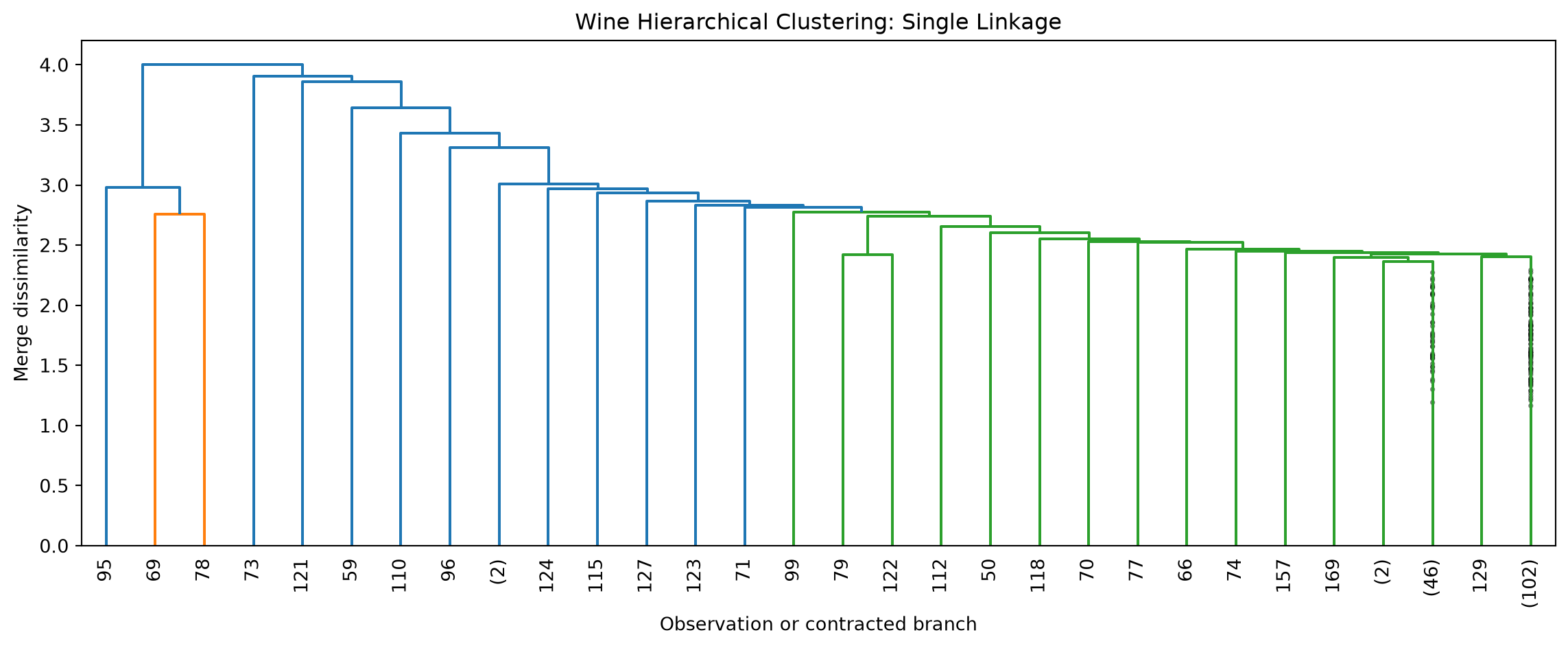
It can recover elongated or irregular connected structures, but it is prone to chaining: a sequence of intermediate points may join otherwise separated dense regions.

Construct a graph connecting points whose distance is below a threshold \(t\). Cutting a single-linkage dendrogram at t gives the connected components of this threshold graph.

Single linkage is also closely related to the minimum spanning tree.

5.2.2. Complete Linkage

\[ d_{\text{complete}}(A,B) = \max_{i\in A,j\in B} d(x_i,x_j). \]

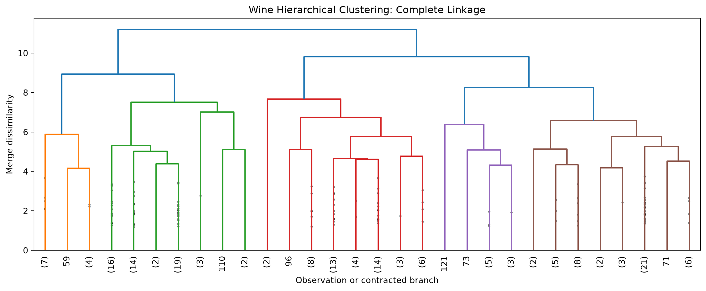
Complete linkage controls the farthest pair across a proposed merge. It tends to form compact clusters with limited diameter.

It is more sensitive than single linkage to extreme pairwise distances.

5.2.3. Average Linkage

\[ d_{\text{average}}(A,B) = \frac{1}{|A||B|} \sum_{i\in A} \sum_{j\in B} d(x_i,x_j). \]

Average linkage balances the nearest-pair behavior of single linkage and the farthest-pair behavior of complete linkage.

5.3. Ward’s Method

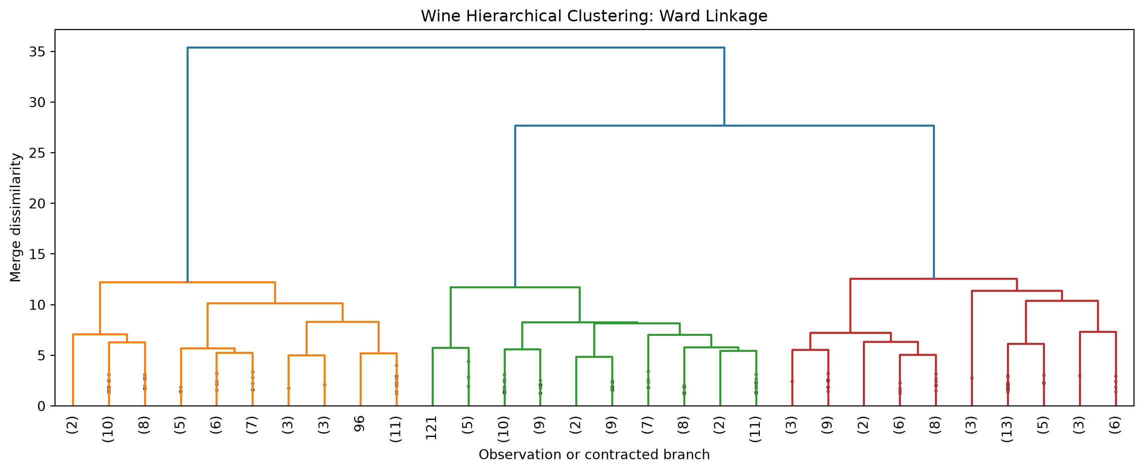
Ward’s method selects the merge causing the smallest increase in total within-cluster squared error.

For a cluster \(C\), define

\[ W(C) = \sum_{i\in C} \|x_i-\mu_C\|^2. \]

The cost of merging A and B is

\[ \Delta(A,B) = W(A\cup B)-W(A)-W(B). \]

NoteTheorem: Ward Merge Cost

For Euclidean data,

\[ \Delta(A,B) = \frac{|A||B|} {|A|+|B|} \|\mu_A-\mu_B\|^2. \]

TipProof

Let \(n_A=|A|, n_B=|B|\), and

\[ \mu_{AB} = \frac{n_A\mu_A+n_B\mu_B} {n_A+n_B}. \]

Using the variance decomposition,

\[ \sum_{i\in A} \|x_i-\mu_{AB}\|^2 = \sum_{i\in A} \|x_i-\mu_A\|^2 + n_A\|\mu_A-\mu_{AB}\|^2. \]

Similarly,

\[ \sum_{i\in B} \|x_i-\mu_{AB}\|^2 = \sum_{i\in B} \|x_i-\mu_B\|^2 + n_B\|\mu_B-\mu_{AB}\|^2. \]

Therefore,

\[ \Delta(A,B) = n_A\|\mu_A-\mu_{AB}\|^2 + n_B\|\mu_B-\mu_{AB}\|^2. \]

Now,

\[ \mu_A-\mu_{AB} = \frac{n_B}{n_A+n_B} (\mu_A-\mu_B), \]

and

\[ \mu_B-\mu_{AB} = -\frac{n_A}{n_A+n_B} (\mu_A-\mu_B). \]

Substituting and simplifying gives

\[ \Delta(A,B) = \frac{n_An_B}{n_A+n_B} \|\mu_A-\mu_B\|^2. \]

Ward’s method is closely connected to the K-means objective but creates a nested greedy hierarchy.

5.4. Interpreting a Dendrogram

A dendrogram should be interpreted through merge heights, not horizontal branch spacing. Cutting it at a height h produces a partition.

Large vertical gaps may suggest comparatively distinct merge levels, but no cut is automatically correct. The hierarchy may reflect:

  • genuine nested structure;
  • gradual continua;
  • batch effects;
  • outlier branches;
  • a linkage artifact.

Clusters extracted from a dendrogram should be examined through their variable profiles and stability.

Hierarchical Clustering

6. Gaussian Mixture Models

6.1. Probabilistic Clustering

A finite mixture model assumes each observation is generated by one of K latent components.

Let \(Z_n\in\{1,\ldots,K\}\) be an unobserved component indicator.

The mixing probabilities satisfy

\[ P(Z_n=k)=\pi_k, \]

where \(\pi_k\geq0, \sum_{k=1}^{K}\pi_k=1\).

Conditional on \(Z_n=k\),

\[ X_n\mid Z_n=k \sim p(x\mid\theta_k). \] The marginal density is

\[ p(x) = \sum_{k=1}^{K} \pi_kp(x\mid\theta_k). \]

Unlike hard clustering, mixture models represent uncertain membership. ### 6.2. Gaussian Mixture Model

In a Gaussian mixture model,

\[ p(x) = \sum_{k=1}^{K} \pi_k \mathcal N(x\mid\mu_k,\Sigma_k). \]

The Gaussian density is

\[ \mathcal N(x\mid\mu_k,\Sigma_k) = \frac{ \exp\left[ -\frac12 (x-\mu_k)^\top \Sigma_k^{-1} (x-\mu_k) \right] }{ (2\pi)^{D/2}|\Sigma_k|^{1/2} }. \]

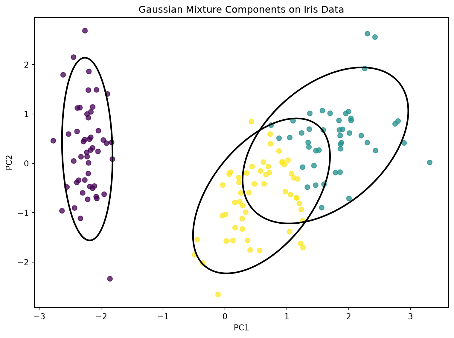
The covariance structure determines component geometry:

  • \(\Sigma_k=\sigma^2I\): equal spherical components;
  • \(\Sigma_k=\sigma_k^2I\): unequal spherical components;
  • shared full covariance: equal elliptical orientation;
  • separate diagonal covariances: axis-aligned ellipses;
  • separate full covariances: flexible ellipsoids.

6.3. Responsibilities

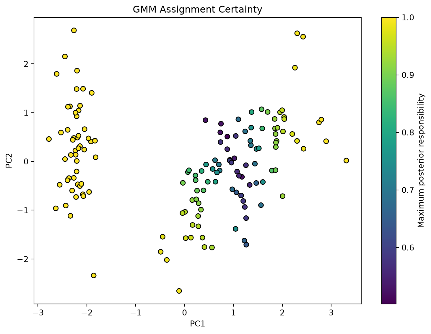
The posterior probability that component k generated observation \(x_n\) is

\[ \gamma_{nk} = P(Z_n=k\mid x_n). \]

By Bayes’ theorem,

\[ \gamma_{nk} = \frac{ \pi_k \mathcal N(x_n\mid\mu_k,\Sigma_k) }{ \sum_{j=1}^{K} \pi_j \mathcal N(x_n\mid\mu_j,\Sigma_j) }. \]

The values satisfy

\[ 0\leq\gamma_{nk}\leq1, \qquad \sum_{k=1}^{K}\gamma_{nk}=1. \]

A hard label can be produced by

\[ \hat z_n=\arg\max_k\gamma_{nk}, \]

but retaining the full responsibility vector reveals ambiguous observations.

6.4. The EM Algorithm for Gaussian Mixtures

The observed-data log-likelihood is

\[ \ell(\Theta) = \sum_{n=1}^{N} \log \left[ \sum_{k=1}^{K} \pi_k \mathcal N(x_n\mid\mu_k,\Sigma_k) \right]. \]

The logarithm of a sum prevents direct componentwise optimization.

Introduce latent indicators

\[ z_{nk}\in\{0,1\}, \qquad \sum_kz_{nk}=1. \] The complete-data log-likelihood is

\[ \ell_c(\Theta) = \sum_{n=1}^{N} \sum_{k=1}^{K} z_{nk} \left[ \log\pi_k+ \log\mathcal N(x_n\mid\mu_k,\Sigma_k) \right]. \] EM alternates:

E-step

Compute

\[ \gamma_{nk} = \mathbb E[z_{nk}\mid x_n,\Theta^{\text{old}}]. \]

M-step

Define effective component counts

\[ N_k = \sum_{n=1}^{N}\gamma_{nk}. \] Then update

\[ \begin{aligned} \pi_k^{\text{new}} &= \frac{N_k}{N},\\ \mu_k^{\text{new}} &= \frac{1}{N_k} \sum_{n=1}^{N} \gamma_{nk}x_n,\\ \Sigma_k^{\text{new}} &= \frac{1}{N_k} \sum_{n=1}^{N} \gamma_{nk} (x_n-\mu_k^{\text{new}}) (x_n-\mu_k^{\text{new}})^\top. \end{aligned} \]

Dempster, Laird, and Rubin formalized EM as a general method for maximum-likelihood estimation with latent or incomplete data1.

TipWhy the EM Likelihood Does Not Decrease

Let \(Z\) denote latent assignments and \(\Theta\) model parameters. For any distribution \(q(Z)\),

\[ \log p(X\mid\Theta) = \mathcal L(q,\Theta) + \operatorname{KL} \left[ q(Z)\| p(Z\mid X,\Theta) \right], \] where \[ \mathcal L(q,\Theta) = \mathbb E_q[\log p(X,Z\mid\Theta)] - \mathbb E_q[\log q(Z)]. \]

Since KL divergence is nonnegative,

\[ \mathcal L(q,\Theta) \leq \log p(X\mid\Theta). \]

The E-step sets

\[ q(Z)=p(Z\mid X,\Theta^{\text{old}}), \] making the bound tight at the current parameters. The M-step increases or maximizes the bound with respect to \(\Theta\). Therefore, the observed-data likelihood cannot decrease.

EM may still converge to a local maximum or saddle point and remains initialization-sensitive.

6.5. Small-Variance Relationship to \(K\)-Means

Consider a Gaussian mixture with equal mixing weights and shared spherical covariance

\[ \Sigma_k=\sigma^2I. \]

The responsibility is proportional to

\[ \gamma_{nk} \propto \exp \left[ -\frac{ \|x_n-\mu_k\|^2 }{ 2\sigma^2 } \right]. \]

As \(\sigma^2\rightarrow0\), the component with the smallest squared distance dominates the exponential sum:

\[ \gamma_{nk} \rightarrow \begin{cases} 1, & k=\arg\min_j\|x_n-\mu_j\|^2,\\ 0, &\text{otherwise}, \end{cases} \]

assuming a unique nearest centroid.

The soft responsibilities become hard nearest-centroid assignments, and the weighted mean update becomes the K-means centroid update.

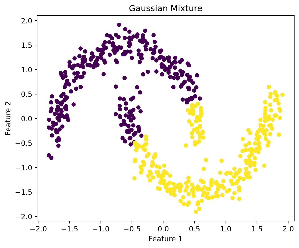
This is more accurately described as a limiting relationship than as a universal equivalence. General Gaussian mixtures can model unequal sizes and elliptical covariance structures that K-means cannot.

WarningMixture Components Are Not Always Substantive Clusters

A mixture component is a probability-density component. It need not correspond one-to-one with a meaningful population group.

A skewed unimodal population may require several Gaussian components for approximation. Conversely, one substantive group may contain several statistical modes.

The component interpretation should therefore be checked against domain variables and posterior ambiguity.

7. Density-Based Clustering

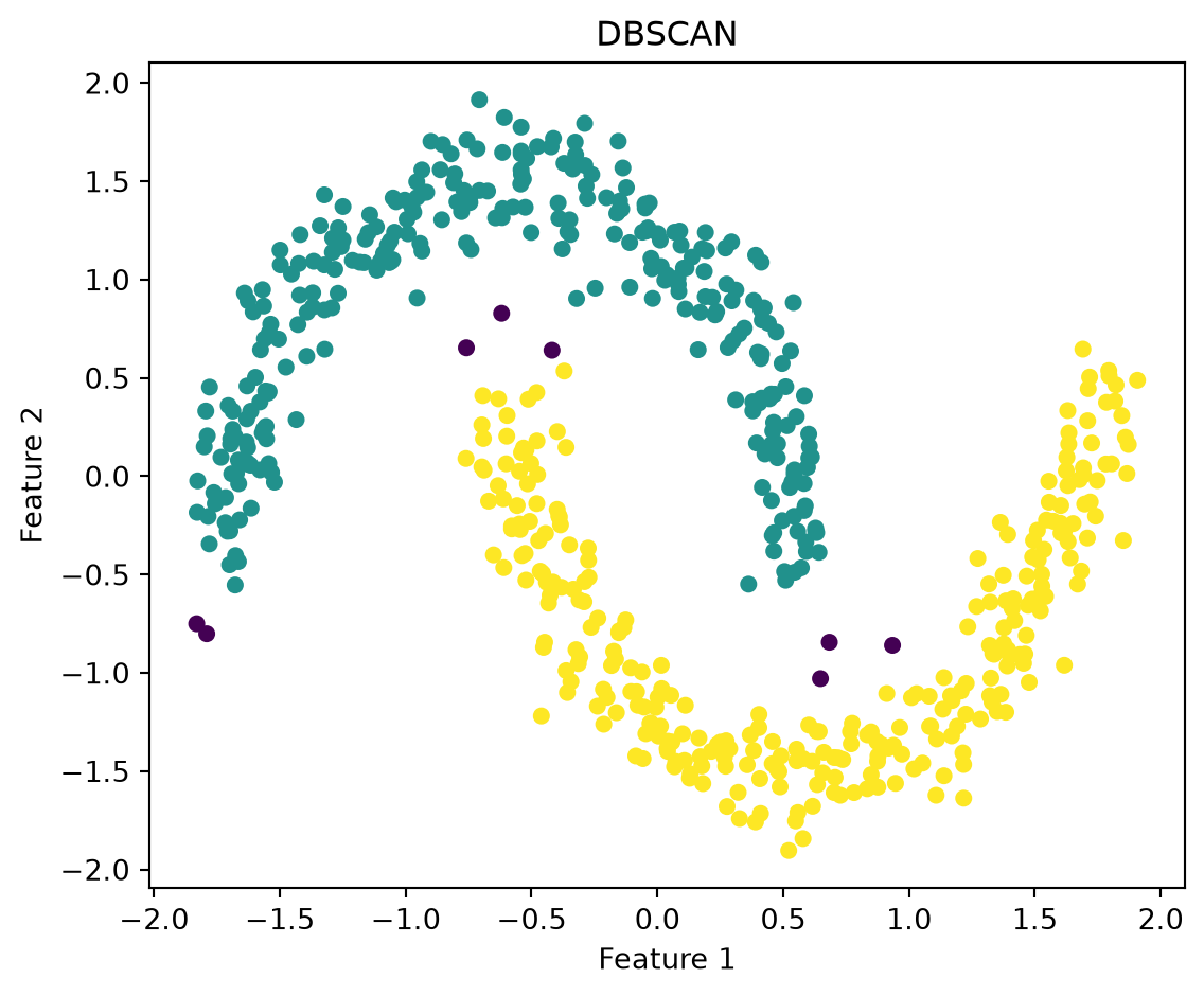
Centroid and Gaussian methods tend to favor convex or elliptical groups. Density-based methods define clusters as connected regions of high observation density separated by low-density regions.

DBSCAN was introduced to discover arbitrarily shaped spatial clusters while identifying isolated points as noise2.

It requires:

  • a neighborhood radius \(\varepsilon>0\);
  • a minimum number of observations \(\operatorname{MinPts}\).

7.1. DBSCAN Definitions

The \(\varepsilon\)-neighborhood of point \(x\) is

\[ N_\varepsilon(x) = \{y:d(x,y)\leq\varepsilon\}. \]

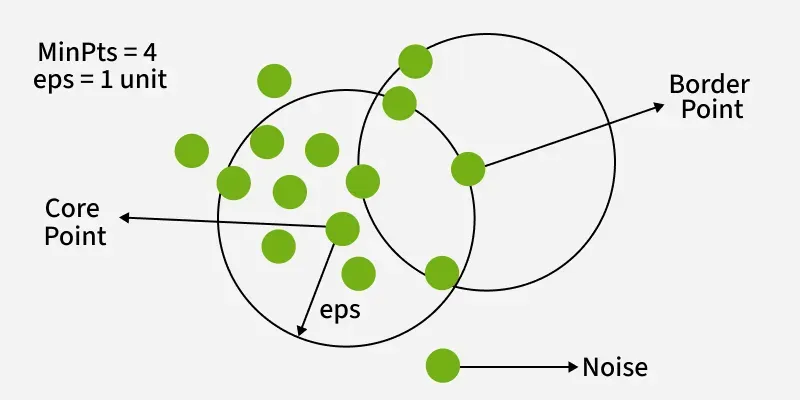
NoteDefinition: Core Point

A point \(x\) is a core point if

\[ |N_\varepsilon(x)| \geq \operatorname{MinPts}. \]

NoteDefinition: Border Point

A point is a border point if it is not a core point but lies in the \(\varepsilon\)-neighborhood of a core point.

NoteDefinition: Noise Point

A point is labeled noise if it is neither a core point nor density-reachable from a core point under the algorithm’s connectivity rules.

Direct density reachability

Point \(y\) is directly density-reachable from \(x\) if

\[ y\in N_\varepsilon(x) \]

and \(x\) is a core point.

Density reachability

Point \(y\) is density-reachable from \(x\) if there is a sequence

\[ x=p_1,p_2,\ldots,p_m=y \]

such that each \(p_{r+1}\) is directly density-reachable from \(p_r\).

A DBSCAN cluster is a maximal density-connected set.

DBSCAN

7.2. DBSCAN Characteristics

Strengths:

  • no requirement to prespecify \(K\);
  • recovery of nonconvex shapes;
  • explicit noise labeling;
  • robustness to isolated observations.

Limitations:

  • sensitivity to \(\varepsilon\) and \(\operatorname{MinPts}\);
  • difficulty with clusters having different densities;
  • degradation in high-dimensional spaces;
  • ambiguous border points;
  • dependence on scale and metric.

A \(k\)-distance plot, which sorts the distance from each point to its \(k\)-th nearest neighbor, can help identify an \(\varepsilon\) transition, though the choice remains judgment-based.

OPTICS and HDBSCAN extend density-based analysis to varying density levels and hierarchical structure.

8. Spectral Clustering

8.1. From Data Points to a Similarity Graph

Spectral clustering represents observations as a graph \(G=(V,E)\), where each vertex corresponds to an observation.

Spectral clustering

Define a nonnegative similarity matrix

\[ W\in\mathbb R^{N\times N}, \]

where \(W_{ij}\) measures similarity between \(x_i\) and \(x_j\).

Common constructions include:

Gaussian similarity

\[ W_{ij} = \exp \left( -\frac{\|x_i-x_j\|^2}{2\sigma^2} \right). \]

\(K\)-nearest-neighbor graph

\[ W_{ij}>0 \]

only when one point is among the k nearest neighbors of the other.

\(\varepsilon\)-neighborhood graph

\[ W_{ij}>0 \quad\text{if}\quad d(x_i,x_j)\leq\varepsilon. \]

Define the degree matrix

\[ D_{ii} = \sum_{j=1}^{N}W_{ij}. \]

8.2. Graph Laplacians

The unnormalized graph Laplacian is \(L=D-W\).

Two normalized forms are

\[ L_{\text{sym}} = I-D^{-1/2}WD^{-1/2}, \]

and

\[ L_{\text{rw}} = I-D^{-1}W. \]

These matrices encode graph connectivity.

NotePositive Semidefiniteness of the Laplacian

If W is symmetric and nonnegative, then

\[ L=D-W \]

is positive semidefinite.

TipProof

For any \(f\in\mathbb R^N\),

\[ f^\top Lf = f^\top Df-f^\top Wf. \]

Because

\[ f^\top Df = \sum_i d_i f_i^2 = \sum_{i,j}W_{ij}f_i^2, \]

and using symmetry,

\[ f^\top Lf = \frac12 \sum_{i,j} W_{ij}(f_i-f_j)^2. \]

Every term is nonnegative, so \(f^\top Lf\geq0\). Therefore, \(L\) is positive semidefinite.

NoteTheorem: Connected Components and Zero Eigenvalues

The number of connected components in an undirected graph equals the multiplicity of eigenvalue 0 of \(L\).

If \(C\) is a connected component and \(\mathbf 1_C\) is its indicator vector, then no edges leave \(C\), and \(L\mathbf 1_C=0.\) Indicators of distinct components are linearly independent. Conversely, any vector satisfying \(Lf=0\) must have \(f_i=f_j\) along every positively weighted edge, because

\[ 0=f^\top Lf = \frac12\sum_{i,j}W_{ij}(f_i-f_j)^2. \]

Thus \(f\) is constant on each connected component.

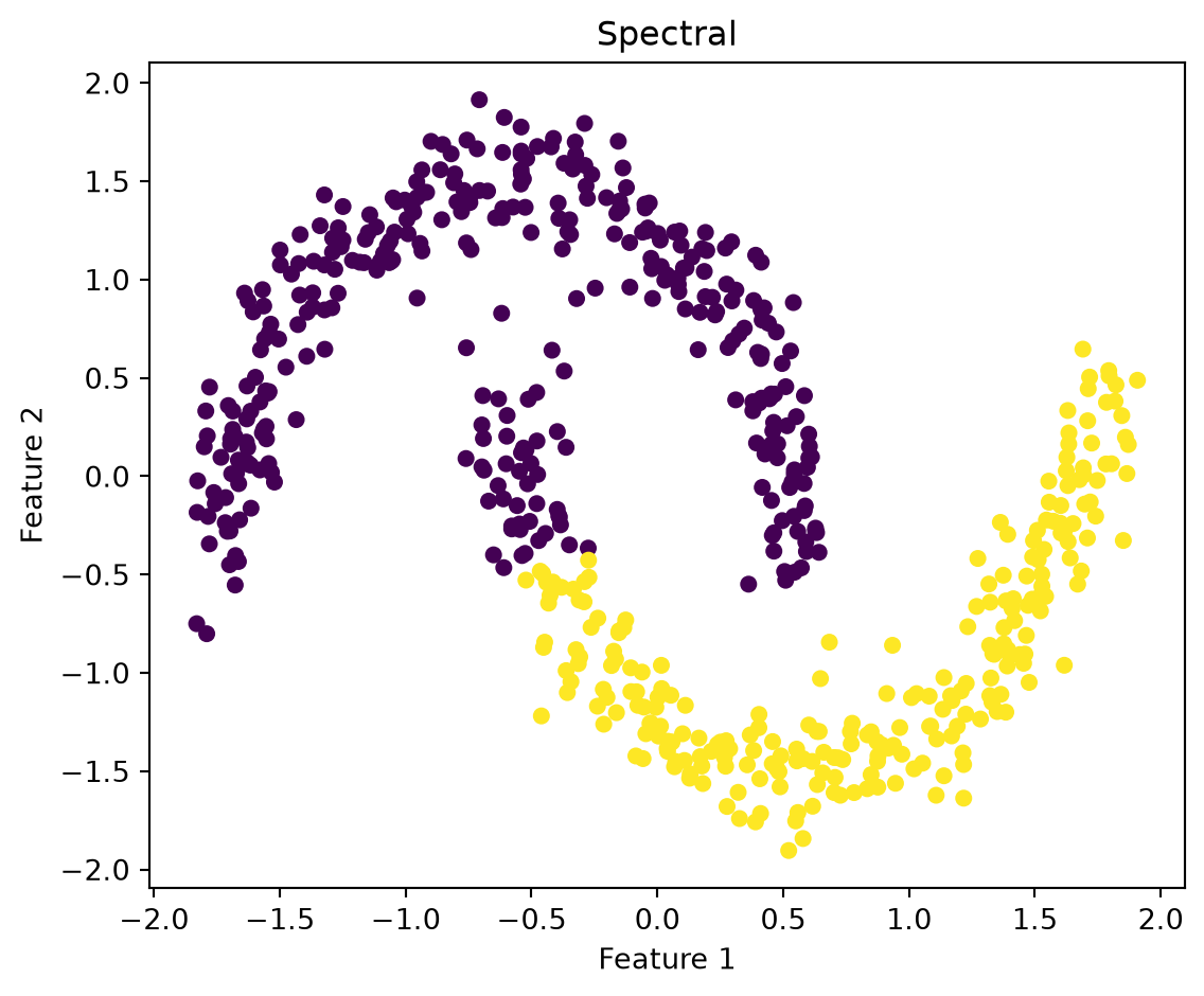
Spectral clustering generalizes this exact result: nearly disconnected graph regions correspond to eigenvectors associated with small eigenvalues.

8.3. Normalized Cut

For disjoint vertex sets \(A\) and \(B\), define

\[ \operatorname{cut}(A,B) = \sum_{i\in A,j\in B}W_{ij}. \]

Define volume

\[ \operatorname{vol}(A) = \sum_{i\in A}d_i. \]

For a bipartition,

\[ \operatorname{Ncut}(A,B) = \frac{\operatorname{cut}(A,B)} {\operatorname{vol}(A)} + \frac{\operatorname{cut}(A,B)} {\operatorname{vol}(B)}. \]

The normalization discourages solutions that isolate a few low-degree vertices.

Exact normalized-cut optimization is combinatorial. Spectral methods relax the discrete indicator constraints into a continuous eigenvector problem. Ng, Jordan, and Weiss developed a widely used normalized spectral clustering algorithm based on leading eigenvectors of a normalized similarity matrix3.

8.4. Spectral Clustering Algorithm

One common version proceeds as follows:

  1. Construct \(W\).
  2. Compute \(D\).
  3. Form

\[ A=D^{-1/2}WD^{-1/2}. \]

  1. Compute the K eigenvectors associated with the largest eigenvalues of \(A\), equivalently the smallest eigenvalues of \(L_{\text{sym}}\).
  2. Stack them into

\[ U\in\mathbb R^{N\times K}. \]

  1. Normalize each row:

\[ Y_{ij} = \frac{U_{ij}} {\left( \sum_{\ell=1}^{K}U_{i\ell}^2 \right)^{1/2}}. \]

  1. Apply \(K\)-means to the row vectors \(Y_i\).

The nonlinear power comes from graph embedding; the final \(K\)-means operates in spectral coordinates rather than the original feature space.

9. Fuzzy Clustering

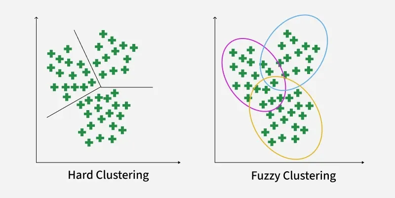
Hard clustering assigns each observation to exactly one group. Fuzzy \(C\)-means assigns membership degrees.

Fuzzy Clustering

Let

\[ u_{nk}\in[0,1], \qquad \sum_{k=1}^{K}u_{nk}=1. \]

The objective is

\[ J_m(U,\mu) = \sum_{n=1}^{N} \sum_{k=1}^{K} u_{nk}^{\,m} \|x_n-\mu_k\|^2, \] where \(m>1\) is the fuzzifier.

For fixed memberships, the centroid update is

\[ \mu_k = \frac{ \sum_{n=1}^{N} u_{nk}^{\,m}x_n }{ \sum_{n=1}^{N} u_{nk}^{\,m} }. \]

For fixed centroids and nonzero distances, membership updates satisfy

\[ u_{nk} = \left[ \sum_{j=1}^{K} \left( \frac{ \|x_n-\mu_k\| }{ \|x_n-\mu_j\| } \right)^{2/(m-1)} \right]^{-1}. \]

As \(m\) approaches 1, memberships become harder. Larger \(m\) produces more diffuse memberships.

Fuzzy membership can be useful when the phenomenon is genuinely gradual—for example, transitional ecological zones or customers with mixed behavioral profiles. It should not be interpreted automatically as a calibrated probability.

10. Topic Models

A scientific article may discuss both machine learning and transportation. A news article may combine economics and public policy. Assigning each document to exactly one topic can be artificial.

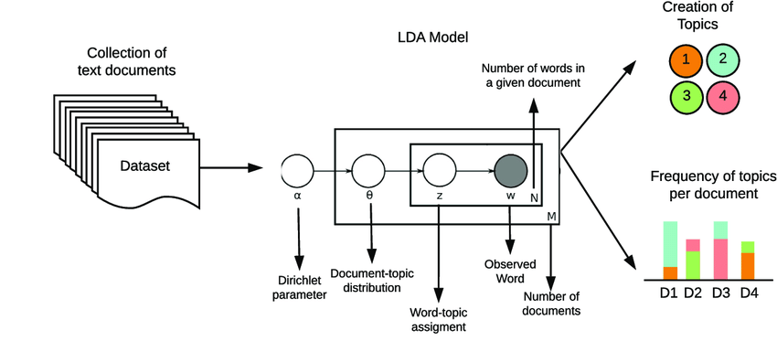
LDA

Latent Dirichlet Allocation represents each document as a distribution over topics and each topic as a distribution over words 4.

Let:

  • \(K\) be the number of topics;
  • \(V\) be vocabulary size;
  • \(\theta_d\) be document \(d\)’s topic proportions;
  • \(\beta_k\) be topic \(k\)’s word distribution.

A common generative construction is:

\[ \theta_d\sim\operatorname{Dirichlet}(\alpha), \]

then for word position \(n\),

\[ \begin{aligned} z_{dn} &\sim \operatorname{Categorical}(\theta_d),\\ w_{dn} &\sim \operatorname{Categorical}(\beta_{z_{dn}}). \end{aligned} \] Each document is therefore a mixture rather than a single cluster.

LDA is not interchangeable with geometric clustering. It is a probabilistic latent-variable model tailored to discrete count data.

11. Self-Organizing Maps

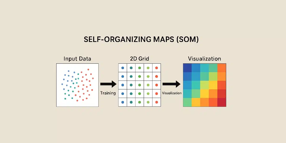
A Self-Organizing Map places prototypes on a fixed low-dimensional grid. Let

\[ m_1,\ldots,m_K\in\mathbb R^D \]

be prototype vectors, each assigned a grid coordinate.

Self-organizing maps

For input \(x\), find the best matching unit

\[ c(x) = \arg\min_k\|x-m_k\|. \]

Update prototype \(k\) by

\[ m_k^{(t+1)} = m_k^{(t)} + \eta_t h_{c(x),k}^{(t)} \left[ x-m_k^{(t)} \right], \]

where:

  • \(\eta_t\) is a learning rate;
  • \(h_{c,k}^{(t)}\) decreases with grid distance from the winning unit.

Unlike ordinary \(K\)-means, nearby prototypes on the grid are updated together. The resulting map attempts to preserve neighborhood structure while providing a two-dimensional visualization.

SOMs are useful exploratory tools but may distort distances and should not be treated as exact low-dimensional geometric embeddings.

12. Archetypal Analysis

\(K\)-means prototypes are central averages. Archetypal analysis instead seeks extreme profiles on or near the convex hull.

Archetypal Analysis

Each observation is approximated as

\[ x_i \approx \sum_{k=1}^{K}\alpha_{ik}z_k, \]

where \(\alpha_{ik}\geq0, \sum_{k=1}^{K}\alpha_{ik}=1\).

Each archetype is itself a convex combination of observations:

\[ z_k = \sum_{j=1}^{N}\beta_{kj}x_j, \]

with \(\beta_{kj}\geq0, \sum_{j=1}^{N}\beta_{kj}=1\).

The objective is

\[ \min_{\alpha,\beta} \sum_{i=1}^{N} \left\| x_i- \sum_{k=1}^{K} \alpha_{ik}z_k \right\|^2. \]

Archetypes describe extreme behavioral or morphological profiles. An observation can be represented as a mixture of these extremes.

13. Incremental and Streaming Clustering

When observations arrive sequentially, storing and refitting on all data may be impractical.

Suppose point \(x_t\) is assigned to cluster \(k\), which has previously received \(n_k\) points. The centroid can be updated by

\[ \mu_k^{\text{new}} = \mu_k^{\text{old}} + \frac{1}{n_k+1} \left( x_t-\mu_k^{\text{old}} \right). \]

This equals the new sample mean.

Mini-batch \(K\)-means uses small batches to approximate Lloyd updates efficiently.

Streaming clustering must also confront concept drift: the population itself may change. A fixed historical cluster may no longer describe current behavior. Forgetting factors or sliding windows can emphasize recent observations.

14. Relational and Graph Clustering

In many datasets, observations are connected:

  • people communicate;
  • airports exchange flights;
  • papers cite one another;
  • customers purchase the same products;
  • proteins interact.

The observations are not independent feature vectors. Their relations carry structural information.

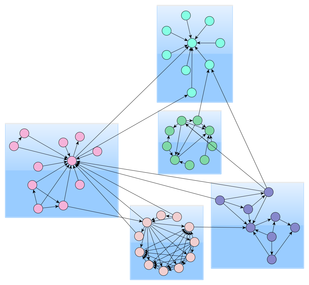
Relational and Graph Clustering

Graph clustering seeks communities with strong internal connectivity and weaker external connectivity. Objectives may include normalized cut, modularity, stochastic block-model likelihood, or random-walk persistence.

A stochastic block model assumes latent group assignments \(z_i\) and connection probabilities

\[ P(A_{ij}=1\mid z_i=k,z_j=\ell) = B_{k\ell}. \]

This is a probabilistic relational analogue of mixture modeling.

Feature information and graph information can also be combined, but their relative weighting must be specified.

15. Internal Evaluation

Internal measures use only the data and fitted partition.

Within-cluster sum of squares

\[ W_K = \sum_{k=1}^{K} \sum_{i\in C_k} \|x_i-\mu_k\|^2. \]

It always weakly decreases as \(K\) increases.

Between-cluster sum of squares

Let \(\bar x = \frac1N\sum_i x_i\).

Define

\[ B_K = \sum_{k=1}^{K} |C_k| \|\mu_k-\bar x\|^2. \]

Total variance decomposition

\[ T=W_K+B_K, \]

where

\[ T = \sum_{i=1}^{N} \|x_i-\bar x\|^2. \]

TipProof of Total Dispersion Decomposition

For \(i\in C_k\),

\[ x_i-\bar x = (x_i-\mu_k)+(\mu_k-\bar x). \]

Squaring,

\[ \|x_i-\bar x\|^2 = \|x_i-\mu_k\|^2 + \|\mu_k-\bar x\|^2 + 2(x_i-\mu_k)^\top(\mu_k-\bar x). \]

Summing within cluster \(k\), the cross-term vanishes because

\[ \sum_{i\in C_k}(x_i-\mu_k)=0. \]

Therefore,

\[ \sum_{i\in C_k}\|x_i-\bar x\|^2 = \sum_{i\in C_k}\|x_i-\mu_k\|^2 + |C_k|\|\mu_k-\bar x\|^2. \]

Summing over clusters gives

\[ T=W_K+B_K. \]

16. External Evaluation

Sometimes known labels exist but are withheld during clustering. They can then evaluate whether the unsupervised partition aligns with an external categorization. This must be interpreted carefully. A clustering solution may be useful without matching known labels, and known labels may not correspond to the geometry being modeled.

16.1. Purity

For cluster \(C_k\), let \(n_{kj}\) be the number of observations with external class \(j\).

Purity is

\[ \operatorname{Purity} = \frac1N \sum_{k=1}^{K} \max_j n_{kj}. \]

Purity tends to increase with the number of clusters and can reach 1 when every observation forms its own cluster. Therefore, it is inadequate alone.

16.2. Rand Index

Consider all \(\binom{N}{2}\) pairs of observations.

Let:

  • \(a\): pairs placed together in both cluster and reference partitions;
  • \(b\): pairs placed apart in both;
  • \(c\): together in clustering but apart in reference;
  • \(d\): apart in clustering but together in reference.

The Rand index is

\[ RI = \frac{a+b}{a+b+c+d}. \]

The Adjusted Rand Index corrects for agreement expected by chance:

\[ ARI = \frac{ \text{observed agreement} - \text{expected agreement} }{ \text{maximum agreement} - \text{expected agreement} }. \]

16.3. Normalized Mutual Information

Let \(C\) be cluster labels and \(Y\) external labels.

Mutual information is

\[ I(C;Y) = \sum_{c,y} p(c,y) \log \frac{p(c,y)}{p(c)p(y)}. \]

One normalization is

\[ NMI(C,Y) = \frac{I(C;Y)} {\sqrt{H(C)H(Y)}}, \]

where \(H(C) = -\sum_c p(c)\log p(c)\).

NMI measures shared information between partitions and is invariant to permutations of cluster labels.

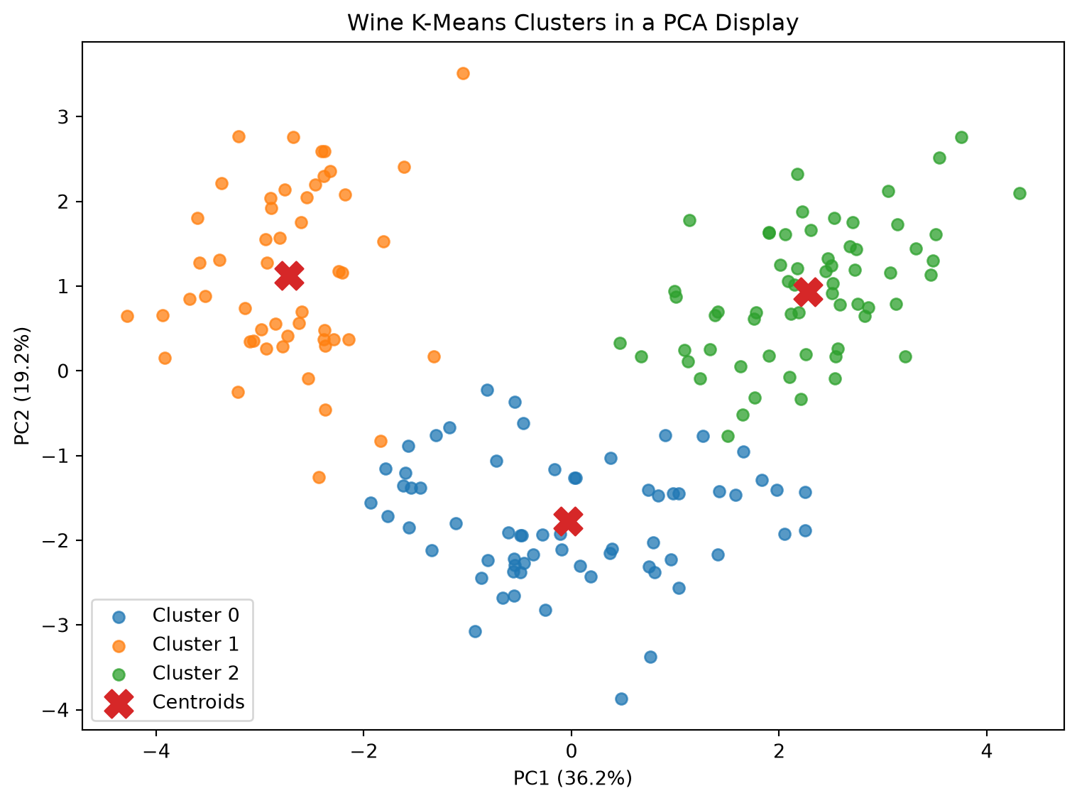
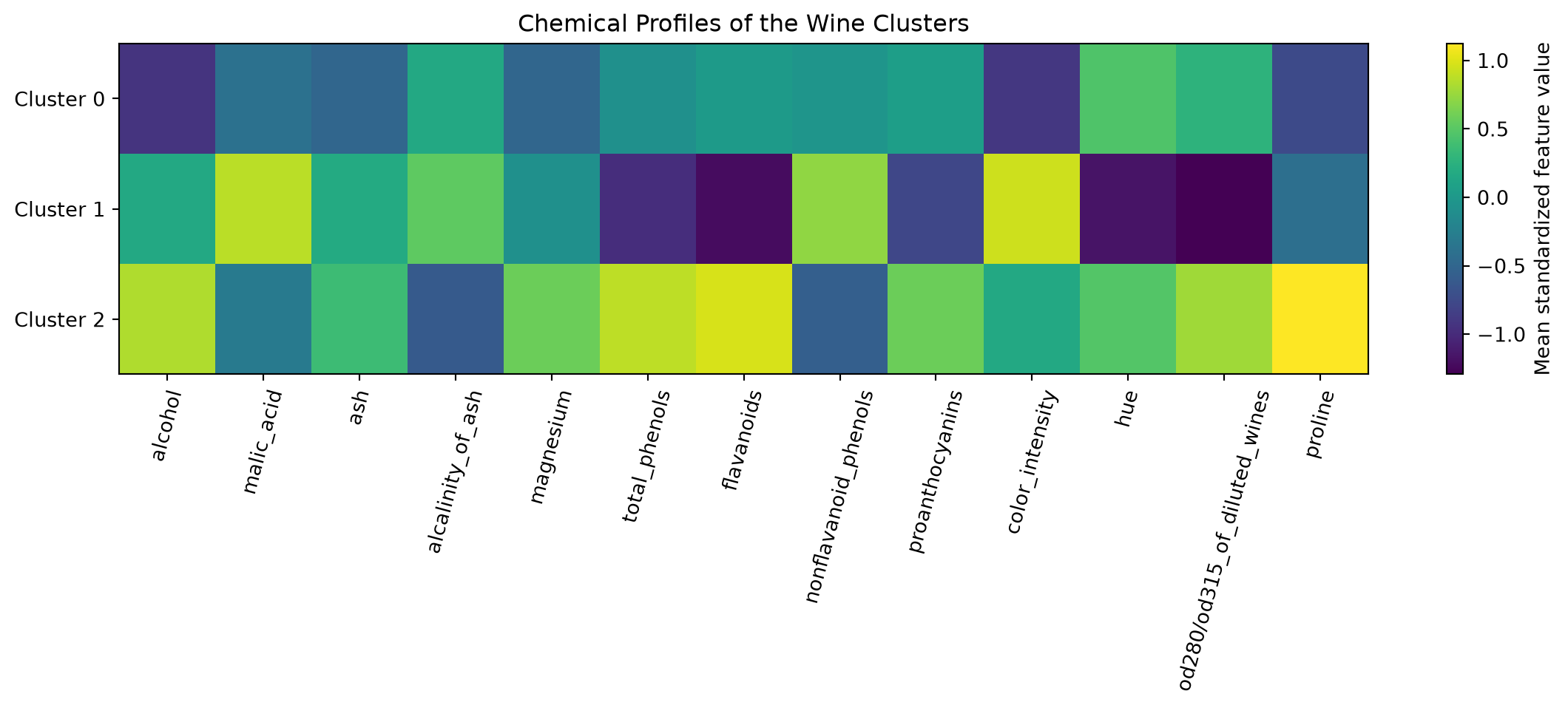
17. Example: Chemical Profiles in the Wine Dataset

Show code
import numpy as np
import pandas as pd
import matplotlib.pyplot as plt

from sklearn.datasets import load_wine
from sklearn.preprocessing import StandardScaler
from sklearn.cluster import KMeans
from sklearn.decomposition import PCA
from sklearn.metrics import (
    silhouette_score,
    silhouette_samples,
    adjusted_rand_score
)

wine = load_wine(as_frame=True)
X_df = wine.data
true_labels = wine.target.to_numpy()

raw_std = X_df.std().sort_values(ascending=False)

plt.figure(figsize=(10, 5))
plt.bar(raw_std.index, raw_std.values)
plt.title("Wine Measurements Before Standardization")
plt.xlabel("Chemical feature")
plt.ylabel("Sample standard deviation")
plt.xticks(rotation=75)
plt.tight_layout()
plt.show()

# Standardize for distance-based clustering
scaler = StandardScaler()
X = scaler.fit_transform(X_df)

k_values = range(2, 11)
inertias = []
silhouettes = []

for k in k_values:
    model = KMeans(
        n_clusters=k,
        n_init=50,
        random_state=42
    )
    labels = model.fit_predict(X)
    inertias.append(model.inertia_)
    silhouettes.append(silhouette_score(X, labels))

plt.figure(figsize=(8, 5))
plt.plot(list(k_values), inertias, marker="o")
plt.title("Wine K-Means Elbow Curve")
plt.xlabel("Number of clusters K")
plt.ylabel("Within-cluster sum of squares")
plt.tight_layout()
plt.show()

plt.figure(figsize=(8, 5))
plt.plot(list(k_values), silhouettes, marker="o")
plt.title("Wine K-Means Average Silhouette")
plt.xlabel("Number of clusters K")
plt.ylabel("Average silhouette coefficient")
plt.tight_layout()
plt.show()

# Fit one chosen solution
k = 3
kmeans = KMeans(
    n_clusters=k,
    n_init=100,
    random_state=42
)
cluster_labels = kmeans.fit_predict(X)

sample_silhouette = silhouette_samples(X, cluster_labels)
average_silhouette = sample_silhouette.mean()

plt.figure(figsize=(8, 6))
y_lower = 10

for cluster_id in range(k):
    values = np.sort(
        sample_silhouette[cluster_labels == cluster_id]
    )

    size = len(values)
    y_upper = y_lower + size

    plt.fill_betweenx(
        np.arange(y_lower, y_upper),
        0,
        values,
        alpha=0.7
    )

    plt.text(
        -0.05,
        y_lower + 0.5 * size,
        str(cluster_id)
    )

    y_lower = y_upper + 10

plt.axvline(
    average_silhouette,
    linestyle="--",
    label=f"Mean = {average_silhouette:.3f}"
)
plt.title("Silhouette Diagram for Wine K-Means")
plt.xlabel("Silhouette coefficient")
plt.ylabel("Clustered observations")
plt.legend()
plt.tight_layout()
plt.show()

pca = PCA(n_components=2)
scores = pca.fit_transform(X)

plt.figure(figsize=(8, 6))

for cluster_id in range(k):
    mask = cluster_labels == cluster_id
    plt.scatter(
        scores[mask, 0],
        scores[mask, 1],
        alpha=0.75,
        label=f"Cluster {cluster_id}"
    )

centers_pca = pca.transform(kmeans.cluster_centers_)
plt.scatter(
    centers_pca[:, 0],
    centers_pca[:, 1],
    marker="X",
    s=220,
    label="Centroids"
)

plt.title("Wine K-Means Clusters in a PCA Display")
plt.xlabel(
    f"PC1 ({pca.explained_variance_ratio_[0]:.1%})"
)
plt.ylabel(
    f"PC2 ({pca.explained_variance_ratio_[1]:.1%})"
)
plt.legend()
plt.tight_layout()
plt.show()

standardized_df = pd.DataFrame(
    X,
    columns=X_df.columns
)
standardized_df["cluster"] = cluster_labels

profiles = standardized_df.groupby("cluster").mean()

plt.figure(figsize=(12, 5))
plt.imshow(profiles, aspect="auto")
plt.colorbar(label="Mean standardized feature value")
plt.xticks(
    range(len(profiles.columns)),
    profiles.columns,
    rotation=75
)
plt.yticks(
    range(len(profiles.index)),
    [f"Cluster {i}" for i in profiles.index]
)
plt.title("Chemical Profiles of the Wine Clusters")
plt.tight_layout()
plt.show()

contingency = pd.crosstab(
    pd.Series(cluster_labels, name="cluster"),
    pd.Series(true_labels, name="cultivar")
)

print("Cluster-by-cultivar table:")
print(contingency)
print(
    "Adjusted Rand Index:",
    adjusted_rand_score(true_labels, cluster_labels)
)

Cluster-by-cultivar table:
cultivar   0   1   2
cluster             
0          0  65   0
1          0   3  48
2         59   3   0
Adjusted Rand Index: 0.8974949815093207

18. Example: Hierarchical Structure in Wine Chemistry

Show code
import matplotlib.pyplot as plt

from scipy.cluster.hierarchy import linkage, dendrogram
from sklearn.datasets import load_wine
from sklearn.preprocessing import StandardScaler

wine = load_wine()
X = StandardScaler().fit_transform(wine.data)

methods = [
    "single",
    "complete",
    "average",
    "ward"
]

for method in methods:
    Z = linkage(
        X,
        method=method,
        metric="euclidean"
    )

    plt.figure(figsize=(12, 5))
    dendrogram(
        Z,
        truncate_mode="lastp",
        p=30,
        leaf_rotation=90,
        show_contracted=True
    )
    plt.title(
        f"Wine Hierarchical Clustering: "
        f"{method.capitalize()} Linkage"
    )
    plt.xlabel("Observation or contracted branch")
    plt.ylabel("Merge dissimilarity")
    plt.tight_layout()
    plt.show()

19. Example: Hard and Soft Clustering

Show code
import numpy as np
import matplotlib.pyplot as plt

from matplotlib.patches import Ellipse
from sklearn.datasets import load_iris
from sklearn.preprocessing import StandardScaler
from sklearn.decomposition import PCA
from sklearn.mixture import GaussianMixture
from sklearn.cluster import KMeans
from sklearn.metrics import adjusted_rand_score

iris = load_iris()
X = StandardScaler().fit_transform(iris.data)
true_labels = iris.target

# Display in two PCA dimensions
pca = PCA(n_components=2)
Z = pca.fit_transform(X)

# Fit models to PCA representation for ellipse visualization
gmm = GaussianMixture(
    n_components=3,
    covariance_type="full",
    n_init=30,
    random_state=42
)
gmm_labels = gmm.fit_predict(Z)
responsibilities = gmm.predict_proba(Z)

kmeans = KMeans(
    n_clusters=3,
    n_init=50,
    random_state=42
)
kmeans_labels = kmeans.fit_predict(Z)

def draw_covariance_ellipse(mean, covariance, ax, n_std=2):
    values, vectors = np.linalg.eigh(covariance)
    order = values.argsort()[::-1]
    values = values[order]
    vectors = vectors[:, order]

    angle = np.degrees(
        np.arctan2(vectors[1, 0], vectors[0, 0])
    )

    width, height = 2 * n_std * np.sqrt(values)

    ellipse = Ellipse(
        xy=mean,
        width=width,
        height=height,
        angle=angle,
        fill=False,
        linewidth=2
    )
    ax.add_patch(ellipse)

fig, ax = plt.subplots(figsize=(8, 6))
ax.scatter(
    Z[:, 0],
    Z[:, 1],
    c=gmm_labels,
    alpha=0.75
)

for mean, covariance in zip(
    gmm.means_,
    gmm.covariances_
):
    draw_covariance_ellipse(
        mean,
        covariance,
        ax
    )

ax.set_title("Gaussian Mixture Components on Iris Data")
ax.set_xlabel("PC1")
ax.set_ylabel("PC2")
plt.tight_layout()
plt.show()

certainty = responsibilities.max(axis=1)

plt.figure(figsize=(8, 6))
scatter = plt.scatter(
    Z[:, 0],
    Z[:, 1],
    c=certainty,
    edgecolor="k"
)
plt.colorbar(
    scatter,
    label="Maximum posterior responsibility"
)
plt.title("GMM Assignment Certainty")
plt.xlabel("PC1")
plt.ylabel("PC2")
plt.tight_layout()
plt.show()

plt.figure(figsize=(8, 6))
plt.scatter(
    Z[:, 0],
    Z[:, 1],
    c=kmeans_labels,
    alpha=0.75
)
plt.scatter(
    kmeans.cluster_centers_[:, 0],
    kmeans.cluster_centers_[:, 1],
    marker="X",
    s=220
)
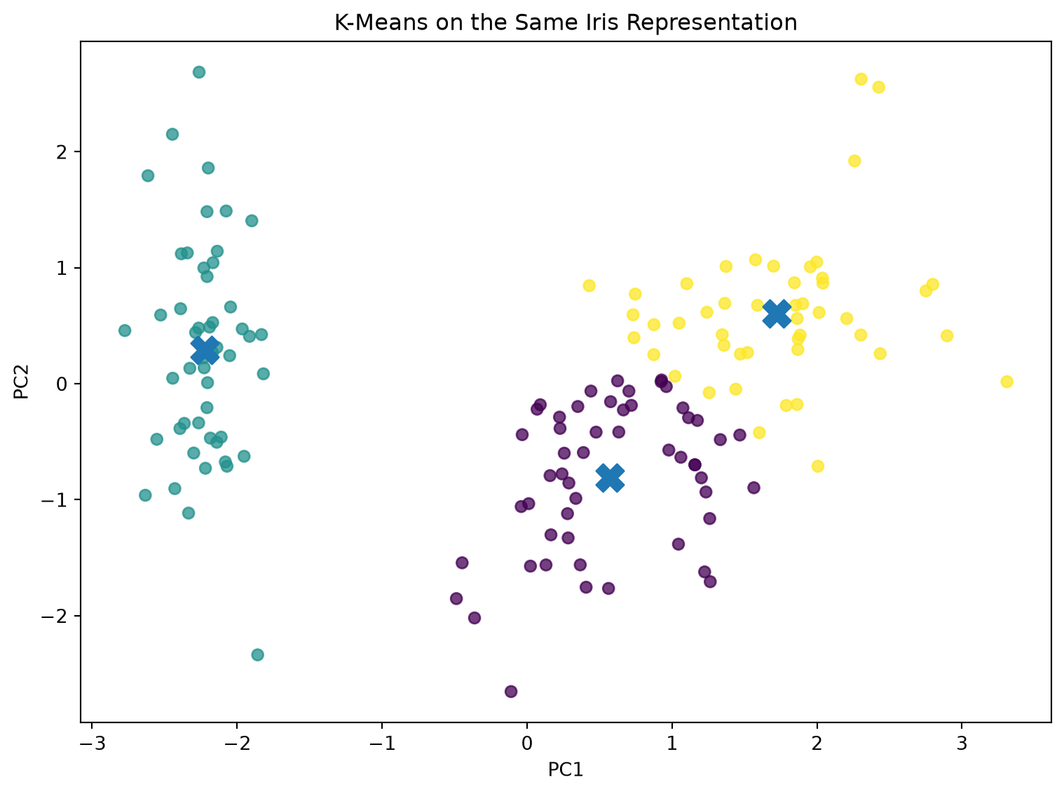
plt.title("K-Means on the Same Iris Representation")
plt.xlabel("PC1")
plt.ylabel("PC2")
plt.tight_layout()
plt.show()

print(
    "External ARI, GMM:",
    adjusted_rand_score(true_labels, gmm_labels)
)
print(
    "External ARI, K-Means:",
    adjusted_rand_score(true_labels, kmeans_labels)
)

External ARI, GMM: 0.6885525109503922
External ARI, K-Means: 0.6201351808870379

20. Example: Image Compression and Segmentation

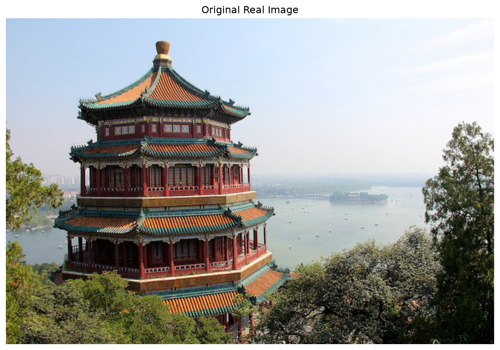
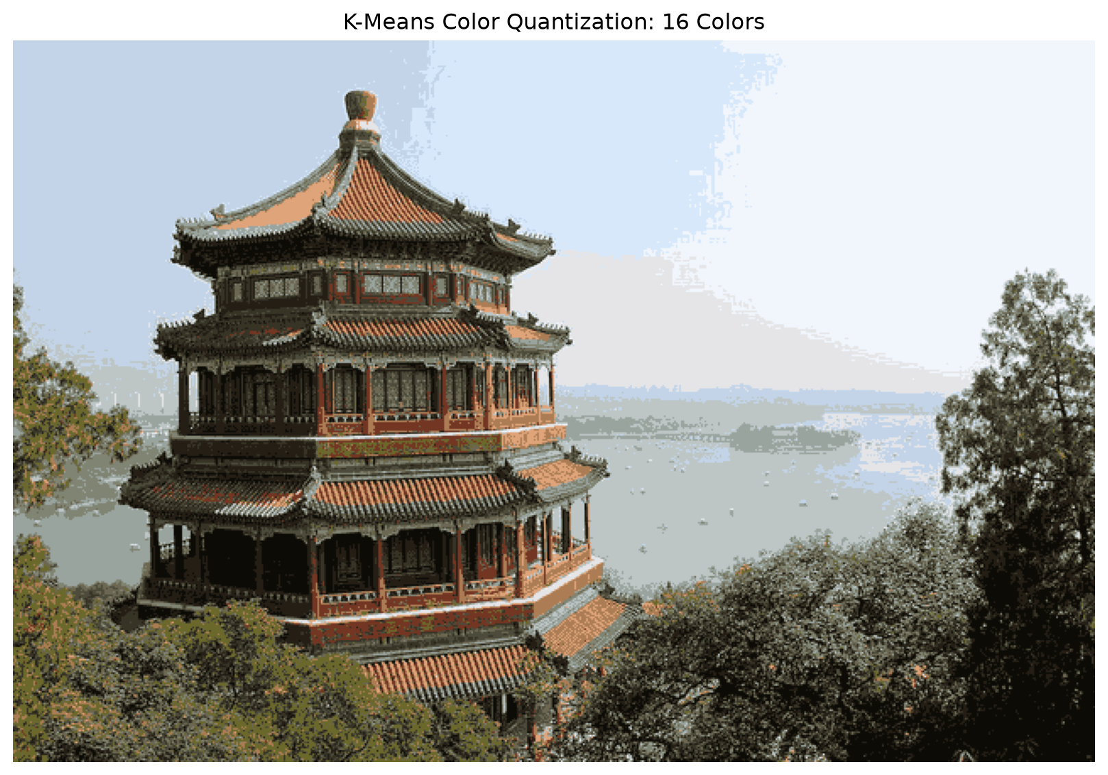
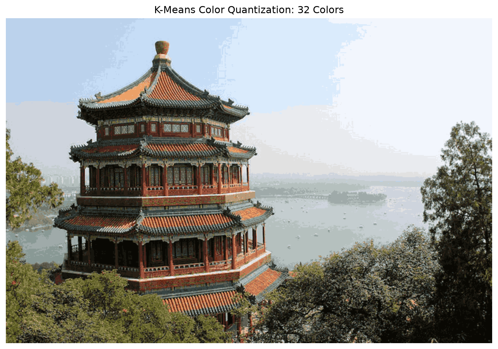
A color image consists of pixels

\[ x_n=(R_n,G_n,B_n)^\top\in\mathbb R^3. \]

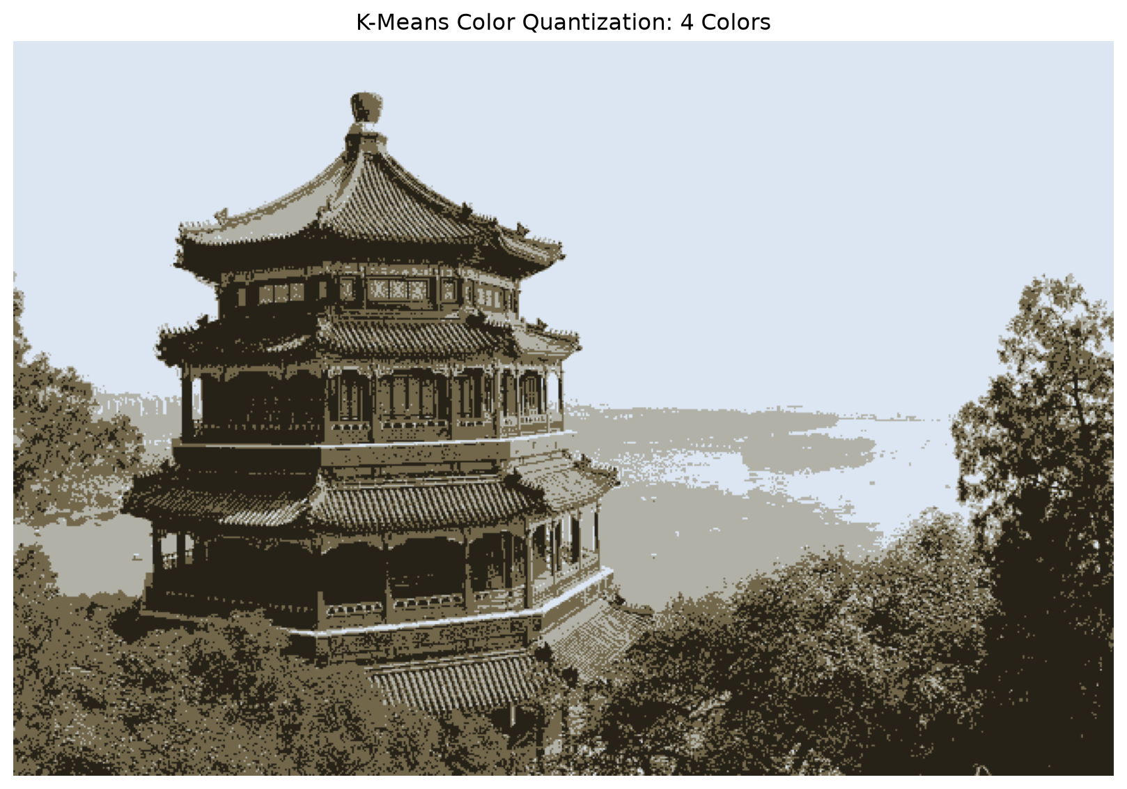
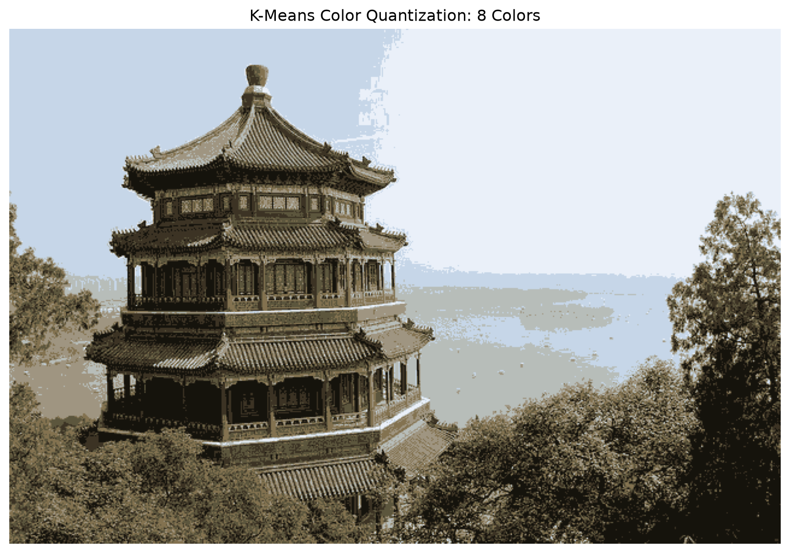
Color quantization uses K-means to replace each pixel color by its nearest centroid. The result uses only K representative colors.

The objective is

\[ \sum_{n=1}^{N} \|x_n-\mu_{z_n}\|^2. \]

This is both clustering and lossy compression.

Show code
import numpy as np
import matplotlib.pyplot as plt

from sklearn.datasets import load_sample_image
from sklearn.cluster import MiniBatchKMeans

image = load_sample_image("china.jpg")
image_float = image.astype(np.float64) / 255.0

height, width, channels = image_float.shape
pixels = image_float.reshape(-1, 3)

# Use a random sample to fit centroids efficiently
rng = np.random.default_rng(42)
sample_size = min(100_000, len(pixels))
sample_indices = rng.choice(
    len(pixels),
    size=sample_size,
    replace=False
)
pixel_sample = pixels[sample_indices]

plt.figure(figsize=(9, 6))
plt.imshow(image_float)
plt.title("Original Real Image")
plt.axis("off")
plt.tight_layout()
plt.show()

for k in [4, 8, 16, 32]:
    model = MiniBatchKMeans(
        n_clusters=k,
        n_init=10,
        random_state=42,
        batch_size=4096
    )

    model.fit(pixel_sample)

    labels = model.predict(pixels)
    compressed_pixels = model.cluster_centers_[labels]
    compressed_image = compressed_pixels.reshape(
        height,
        width,
        channels
    )

    plt.figure(figsize=(9, 6))
    plt.imshow(
        np.clip(compressed_image, 0, 1)
    )
    plt.title(f"K-Means Color Quantization: {k} Colors")
    plt.axis("off")
    plt.tight_layout()
    plt.show()

palette_model = MiniBatchKMeans(
    n_clusters=16,
    n_init=10,
    random_state=42,
    batch_size=4096
)
palette_model.fit(pixel_sample)

palette = palette_model.cluster_centers_

plt.figure(figsize=(10, 2))
plt.imshow(palette.reshape(1, -1, 3))
plt.title("Learned 16-Color Prototype Palette")
plt.yticks([])
plt.xticks(range(16))
plt.tight_layout()
plt.show()

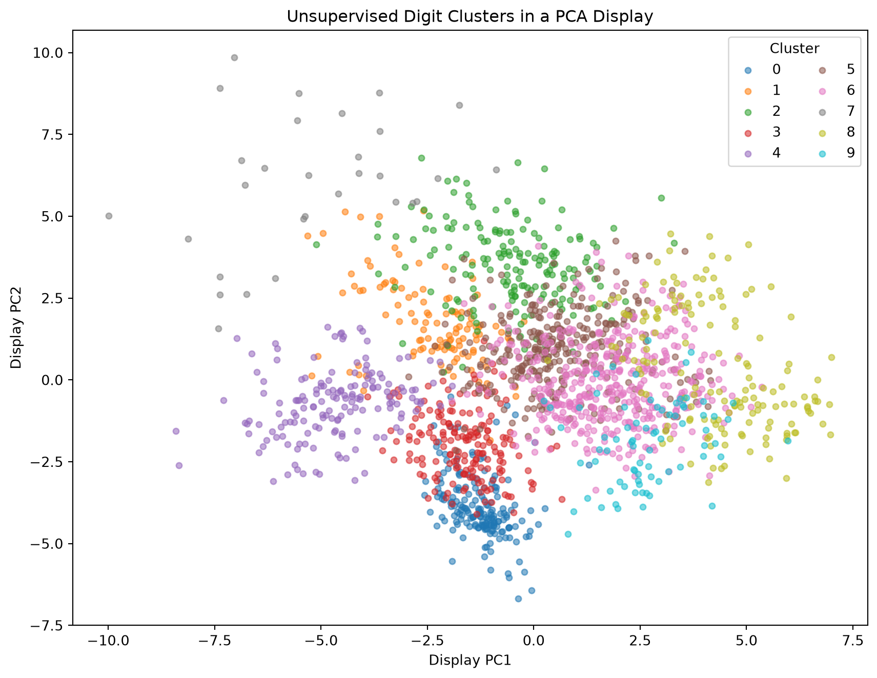
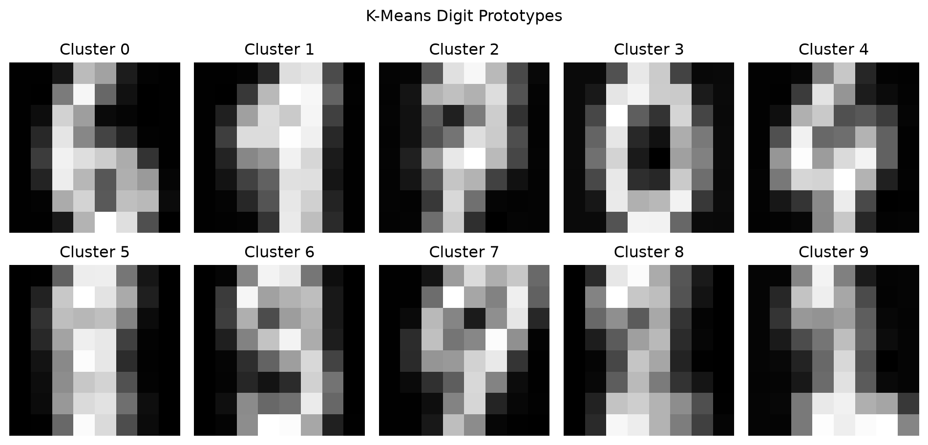
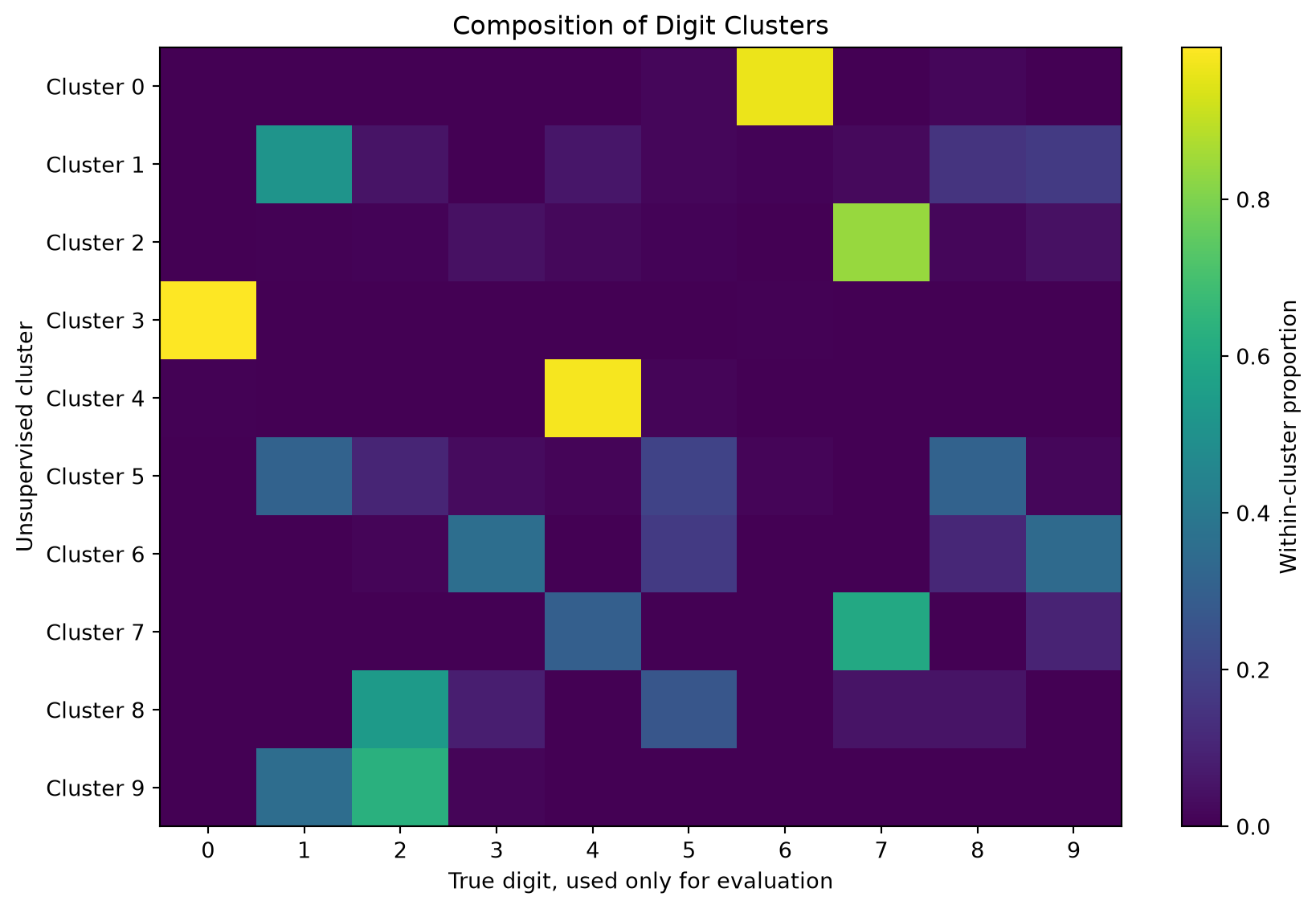
21. Example: Clustering Handwritten Digits

Each \(8\times8\) digit image is represented by a vector

\[ x_n\in\mathbb R^{64}. \]

The clustering algorithm receives only pixel intensities. True digit labels are used afterward to inspect alignment.

Show code
import numpy as np
import pandas as pd
import matplotlib.pyplot as plt

from sklearn.datasets import load_digits
from sklearn.preprocessing import StandardScaler
from sklearn.decomposition import PCA
from sklearn.cluster import KMeans
from sklearn.metrics import (
    adjusted_rand_score,
    normalized_mutual_info_score,
    silhouette_score
)

digits = load_digits()
X_raw = digits.data
true_digits = digits.target

# Scale pixels for this geometric analysis
X = StandardScaler().fit_transform(X_raw)

# Reduce moderate noise before clustering
pca_model = PCA(
    n_components=0.90,
    random_state=42
)
X_reduced = pca_model.fit_transform(X)

kmeans = KMeans(
    n_clusters=10,
    n_init=100,
    random_state=42
)
clusters = kmeans.fit_predict(X_reduced)

display_pca = PCA(n_components=2)
Z = display_pca.fit_transform(X)

plt.figure(figsize=(9, 7))

for cluster_id in range(10):
    mask = clusters == cluster_id
    plt.scatter(
        Z[mask, 0],
        Z[mask, 1],
        s=18,
        alpha=0.55,
        label=str(cluster_id)
    )

plt.title("Unsupervised Digit Clusters in a PCA Display")
plt.xlabel("Display PC1")
plt.ylabel("Display PC2")
plt.legend(
    title="Cluster",
    ncol=2
)
plt.tight_layout()
plt.show()

centers_standardized = pca_model.inverse_transform(
    kmeans.cluster_centers_
)

# Undo StandardScaler manually
scaler = StandardScaler().fit(X_raw)
# Refit properly for clear inverse transform pipeline below
X_scaled = scaler.transform(X_raw)
pca_model_2 = PCA(n_components=0.90, random_state=42)
X_reduced_2 = pca_model_2.fit_transform(X_scaled)
kmeans_2 = KMeans(
    n_clusters=10,
    n_init=100,
    random_state=42
).fit(X_reduced_2)

centers_scaled = pca_model_2.inverse_transform(
    kmeans_2.cluster_centers_
)
centers_pixels = scaler.inverse_transform(
    centers_scaled
)

plt.figure(figsize=(10, 5))

for cluster_id in range(10):
    plt.subplot(2, 5, cluster_id + 1)
    plt.imshow(
        centers_pixels[cluster_id].reshape(8, 8),
        cmap="gray"
    )
    plt.title(f"Cluster {cluster_id}")
    plt.axis("off")

plt.suptitle("K-Means Digit Prototypes")
plt.tight_layout()
plt.show()

composition = pd.crosstab(
    pd.Series(kmeans_2.labels_, name="cluster"),
    pd.Series(true_digits, name="digit"),
    normalize="index"
)

plt.figure(figsize=(9, 6))
plt.imshow(
    composition,
    aspect="auto"
)
plt.colorbar(
    label="Within-cluster proportion"
)
plt.xticks(
    range(10),
    range(10)
)
plt.yticks(
    range(10),
    [f"Cluster {i}" for i in range(10)]
)
plt.xlabel("True digit, used only for evaluation")
plt.ylabel("Unsupervised cluster")
plt.title("Composition of Digit Clusters")
plt.tight_layout()
plt.show()

print(
    "Silhouette:",
    silhouette_score(
        X_reduced_2,
        kmeans_2.labels_,
        sample_size=1000,
        random_state=42
    )
)

print(
    "Adjusted Rand Index:",
    adjusted_rand_score(
        true_digits,
        kmeans_2.labels_
    )
)

print(
    "Normalized Mutual Information:",
    normalized_mutual_info_score(
        true_digits,
        kmeans_2.labels_
    )
)

Silhouette: 0.17271895397874237
Adjusted Rand Index: 0.4646456035374872
Normalized Mutual Information: 0.6228507417700094

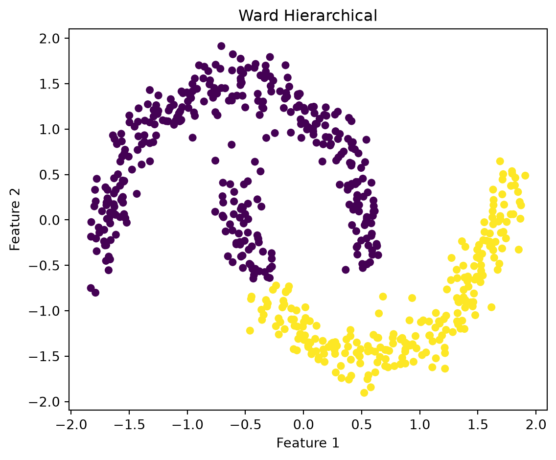
22. Comparing Algorithms on Nonconvex Structure

Show code
import matplotlib.pyplot as plt

from sklearn.datasets import make_moons
from sklearn.preprocessing import StandardScaler
from sklearn.cluster import (
    KMeans,
    AgglomerativeClustering,
    DBSCAN,
    SpectralClustering
)
from sklearn.mixture import GaussianMixture

X, _ = make_moons(
    n_samples=600,
    noise=0.08,
    random_state=42
)
X = StandardScaler().fit_transform(X)

models = {
    "K-Means": KMeans(
        n_clusters=2,
        n_init=30,
        random_state=42
    ),
    "Ward Hierarchical": AgglomerativeClustering(
        n_clusters=2,
        linkage="ward"
    ),
    "Gaussian Mixture": GaussianMixture(
        n_components=2,
        covariance_type="full",
        n_init=20,
        random_state=42
    ),
    "DBSCAN": DBSCAN(
        eps=0.22,
        min_samples=8
    ),
    "Spectral": SpectralClustering(
        n_clusters=2,
        affinity="nearest_neighbors",
        n_neighbors=15,
        assign_labels="kmeans",
        random_state=42
    )
}

for name, model in models.items():
    labels = model.fit_predict(X)

    plt.figure(figsize=(6, 5))
    plt.scatter(
        X[:, 0],
        X[:, 1],
        c=labels,
        s=25
    )
    plt.title(name)
    plt.xlabel("Feature 1")
    plt.ylabel("Feature 2")
    plt.tight_layout()
    plt.show()


Clustering is not a single algorithmic operation but a family of unsupervised approaches for expressing structure in unlabeled data.

\(K\)-means defines clusters through squared Euclidean compactness:

\[ \min \sum_{n=1}^{N} \sum_{k=1}^{K} z_{nk}\|x_n-\mu_k\|^2. \]

Lloyd’s algorithm alternates between nearest-centroid assignment and mean updates. Each step decreases the objective, but the nonconvex problem permits local optima and initialization dependence.

\(K\)-medoids replaces abstract means with observed representatives and supports more general dissimilarities. Hierarchical clustering reveals nested relationships, but the result depends critically on linkage. Ward’s method joins groups according to the increase

\[ \frac{|A||B|}{|A|+|B|} \|\mu_A-\mu_B\|^2 \]

in within-cluster variation.

Gaussian mixture models treat clusters as latent probability components. Their responsibilities

\[ \gamma_{nk} = P(Z_n=k\mid x_n) \]

retain assignment uncertainty. EM alternates between estimating these responsibilities and updating component parameters. K-means emerges as a small-variance limiting case of an equal spherical Gaussian mixture, but general mixture models are more flexible.

DBSCAN identifies density-connected regions and explicitly labels noise. Spectral clustering transforms similarity into graph geometry and uses Laplacian eigenvectors to reveal weakly connected graph regions. Fuzzy clustering and topic models allow mixed membership, while SOMs, archetypal analysis, streaming methods, and relational models adapt the clustering idea to specialized structures.

The absence of labels makes evaluation fundamentally difficult. WCSS, silhouettes, and gap statistics measure properties induced by specific objectives. External measures such as ARI and NMI require labels that were not used in fitting. Stability and independent cluster characterization are therefore essential.

The deepest lesson is that a cluster is not simply found in data. It is defined jointly by:

  • the observation unit;
  • the selected variables;
  • data transformations;
  • the metric or likelihood;
  • the clustering objective;
  • the number of groups or density scale;
  • the sampling context;
  • the intended interpretation.

Clustering is most useful when these choices are made explicitly and when the resulting groups remain stable, interpretable, and appropriate for the decisions they are meant to support.

Next chapter: Debugging and Evaluating

Footnotes

  1. Dempster, A. P., N. M. Laird, and D. B. Rubin. “Maximum Likelihood from Incomplete Data Via the EM Algorithm.” Journal of the Royal Statistical Society: Series B (Methodological) 39, no. 1 (1977): 1–22. https://doi.org/10.1111/j.2517-6161.1977.tb01600.x.↩︎
  2. Ester, Martin, Hans-Peter Kriegel, Jörg Sander, and Xiaowei Xu. “A Density-Based Algorithm for Discovering Clusters in Large Spatial Databases with Noise.” Proceedings of the Second International Conference on Knowledge Discovery and Data Mining (Portland, Oregon), KDD’96, August 2, 1996, 226–31.↩︎
  3. Ng, Andrew, Michael Jordan, and Yair Weiss. “On Spectral Clustering: Analysis and an Algorithm.” Advances in Neural Information Processing Systems 14 (2001). https://proceedings.neurips.cc/paper_files/paper/2001/hash/801272ee79cfde7fa5960571fee36b9b-Abstract.html.↩︎
  4. Blei, David M., Andrew Y. Ng, and Michael I. Jordan. “Latent Dirichlet Allocation.” The Journal of Machine Learning Research 3, no. null (2003): 993–1022.↩︎