Data Modeling - SVM

So far, we have known that regression models estimate explicit functional relationships, tree-based models recursively partition the feature space, and K-Nearest Neighbors predicts from local similarity. Support Vector Machines, or SVMs, introduce a different perspective: classification and regression through maximum-margin optimization.

An SVM searches for a boundary that separates classes while maintaining the largest possible margin from the nearest training observations. The nearest observations are called support vectors, because they determine the position and orientation of the final decision boundary.

For binary classification, the basic SVM problems begins with data \(\mathcal D_n=\{(x_i, y_i\}_{i=1}^n\) where \(x_i\in \mathbb R^p\) and \(y_i\in \{-1, +1\}\). The classifier is based on a decision function

\[ f(x) = w^\top x + b \]

The predicted class is

\[ \hat y(x) = \text{sign}(f(x)) \]

The separating hyperplane is

\[ w^\top x + b = 0 \]

So the central mathematical question is:

Among all hyperplanes that separate the classes, which one has the largest margin?

This question leads to a convex quadratic optimization problem. The maximum-margin formulation makes SVMs different from models such as logistic regression. Logistic regression estimates class probabilities through a likelihood model, while SVMs focus on geometric separation and margin maximization.

Historically, SVMs are connected to statistical learning theory and the principle of Structural Risk Minimization, or SRM. Instead of minimizing training error alone, SRM seeks to control model complexity in order to improve generalization. In SVMs, this control appears through the margin and regularization terms.

1. Geometric Foundations

1.1. Hyperplanes

NoteDefinition: Hyperplanes

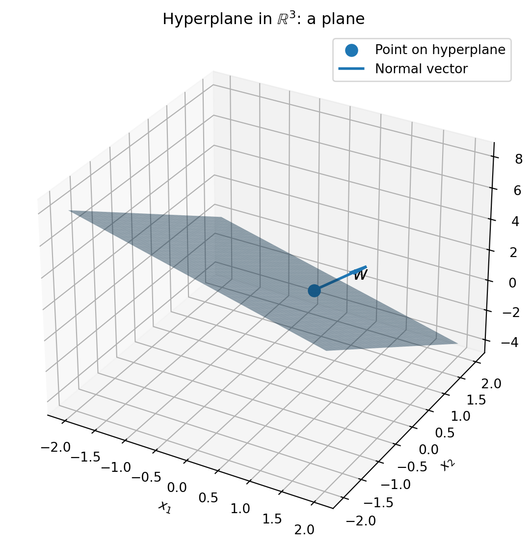
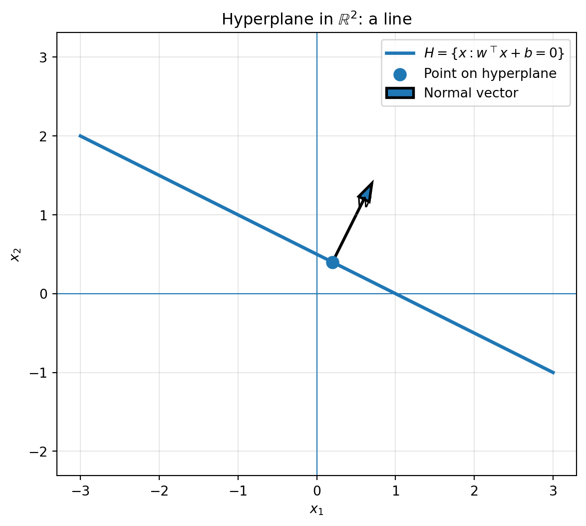
A hyperplane in \(\mathbb R^p\) is the set

\[ H=\{x\in \mathbb R^p: w^\top x+ b = 0\}, \]

where \(w\in \mathbb R^p\) is the normal vector and \(b\in \mathbb R\) is the intercept.

The vector \(w\) in perpendicular to the hyperplane. The sign of \(w^\top x + b\) determines on which side of the hyperplane the point \(x\) lies.

Thus, a linear binary classifier is

\[ \hat y(x) = \begin{cases}+1, & w^\top x + b \geq 0\\ -1,& w^\top x+b <0 \end{cases} \]

Equivalently,

\[ \hat y(x) = \text{sign}(w^\top x+b) \]

import numpy as np
import matplotlib.pyplot as plt

def closest_point_on_hyperplane(w, b):
    """
    Return the point on H closest to the origin.

    H = {x : w^T x + b = 0}

    The closest point is:
        x0 = -b * w / ||w||^2
    """
    w = np.array(w, dtype=float)
    return -b * w / np.dot(w, w)
    
w = np.array([1, 2])
b = -1

x1 = np.linspace(-3, 3, 200)
x2 = -(w[0] * x1 + b) / w[1]

x0 = closest_point_on_hyperplane(w, b)

plt.figure(figsize=(7, 6))

# Plot hyperplane
plt.plot(x1, x2, linewidth=2.5, label=r"$H=\{x:w^\top x+b=0\}$")

# Plot closest point on the hyperplane
plt.scatter(x0[0], x0[1], s=80, zorder=5, label="Point on hyperplane")

# Plot normal vector
plt.arrow(
    x0[0], x0[1],
    w[0] * 0.5, w[1] * 0.5,
    head_width=0.15,
    length_includes_head=True,
    linewidth=2,
    label="Normal vector"
)

plt.text(
    x0[0] + 0.3,
    x0[1] + 0.7,
    r"$w$",
    fontsize=14
)

plt.axhline(0, linewidth=0.8)
plt.axvline(0, linewidth=0.8)

plt.xlabel(r"$x_1$")
plt.ylabel(r"$x_2$")
plt.title(r"Hyperplane in $\mathbb{R}^2$: a line")
plt.grid(alpha=0.3)
plt.axis("equal")
plt.legend()
plt.show()

from mpl_toolkits.mplot3d import Axes3D

w = np.array([1, 2, 1])
b = -2

x1 = np.linspace(-2, 2, 40)
x2 = np.linspace(-2, 2, 40)

X1, X2 = np.meshgrid(x1, x2)

# Solve w1*x1 + w2*x2 + w3*x3 + b = 0
X3 = -(w[0] * X1 + w[1] * X2 + b) / w[2]

x0 = closest_point_on_hyperplane(w, b)

fig = plt.figure(figsize=(9, 7))
ax = fig.add_subplot(111, projection="3d")

# Plot plane
ax.plot_surface(X1, X2, X3, alpha=0.45)

# Plot closest point on plane
ax.scatter(
    x0[0], x0[1], x0[2],
    s=80,
    label="Point on hyperplane"
)

# Plot normal vector
ax.quiver(
    x0[0], x0[1], x0[2],
    w[0], w[1], w[2],
    length=1.0,
    normalize=True,
    linewidth=2,
    label="Normal vector"
)

ax.text(
    x0[0] + 0.4,
    x0[1] + 0.4,
    x0[2] + 0.4,
    r"$w$",
    fontsize=14
)

ax.set_xlabel(r"$x_1$")
ax.set_ylabel(r"$x_2$")
ax.set_zlabel(r"$x_3$")

ax.set_title(r"Hyperplane in $\mathbb{R}^3$: a plane")
ax.legend()

plt.show()

1.2. Functional Margin

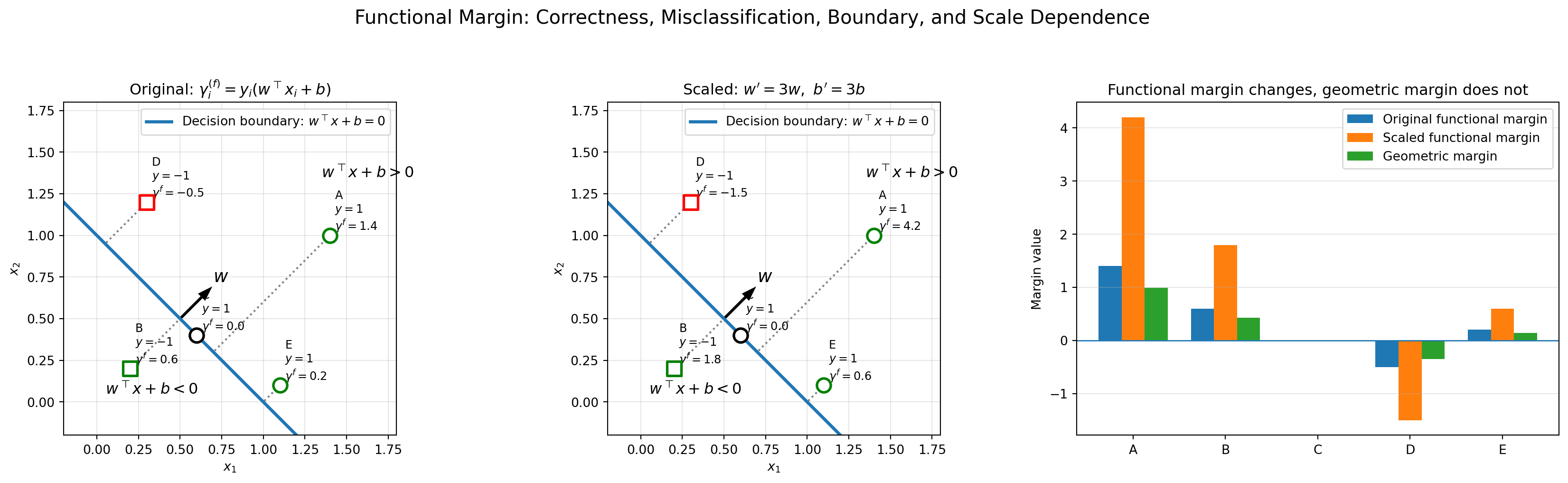
For a labeled observation \((x_i, y_i)\), define the functional margin as

\[ \gamma_i^{(f)} = y_i(w^\top x_i + b). \]

• If \(\gamma_i^{(f)}>0\) then \(x_i\) is correctly classified.
• If \(\gamma_i^{(f)} <0\) then \(x_i\) is misclassified.
• If \(\gamma_i^{(f)} = 0\) then \(x_i\) lies exactly on the decision boundary.

However, the functional margin is not scale-invariant. If we multiply \(w\) and \(b\) by a positive constant \(a>0\), then

\[ w' = aw, \quad b' = ab \]

and

\[ y_i((aw)^\top x_i+ab) = ay_i(w^\top x_i + b). \]

Thus, the functional margin changes even though the separating hyperplane itself does not. To define a meaningful geometric margin, we must normalize by \(||w||\).

1.3. Geometric Margin

The signed distance from a point \(x_i\) to the hyperplane \(w^\top x+b =0\) is

\[ \frac{w^\top x_i+b}{||w||}. \]

Including the class label gives the geometric margin:

\[ \gamma_i = \frac{y_i(w^\top x_i+b)}{||w||} \]

The margin of the classifier is the minimum geometric margin over all training observations:

\[ \gamma = \min_{i=1,\dots, n} \frac{y_i(w^\top x_i+b)}{||w||} \]

The maximum-margin classifier chooses \(w\) and \(b\) to maximize \(\gamma\).

import numpy as np
import matplotlib.pyplot as plt

# Define a simple 2D example

# Hyperplane:
# w^T x + b = 0
# x1 + x2 - 1 = 0

w = np.array([1.0, 1.0])
b = -1.0

# Scale factor
a = 3.0

w_scaled = a * w
b_scaled = a * b

# Points and labels
# y = +1 means the point should be above the boundary
# y = -1 means the point should be below the boundary

X = np.array([
    [1.4, 1.0],   # correctly classified positive
    [0.2, 0.2],   # correctly classified negative
    [0.6, 0.4],   # exactly on boundary
    [0.3, 1.2],   # misclassified negative
    [1.1, 0.1],   # correctly classified positive
])

y = np.array([1, -1, 1, -1, 1])

point_names = ["A", "B", "C", "D", "E"]

def decision_score(X, w, b):
    """
    Compute f(x) = w^T x + b.
    """
    return X @ w + b


def functional_margin(X, y, w, b):
    """
    gamma_i^(f) = y_i (w^T x_i + b)
    """
    return y * decision_score(X, w, b)


def geometric_margin(X, y, w, b):
    """
    gamma_i = y_i (w^T x_i + b) / ||w||
    """
    return functional_margin(X, y, w, b) / np.linalg.norm(w)


def project_to_hyperplane(x, w, b):
    """
    Project a point x onto the hyperplane w^T x + b = 0.
    """
    return x - ((w @ x + b) / np.dot(w, w)) * w
    
gamma_original = functional_margin(X, y, w, b)
gamma_scaled = functional_margin(X, y, w_scaled, b_scaled)

geo_original = geometric_margin(X, y, w, b)
geo_scaled = geometric_margin(X, y, w_scaled, b_scaled)

print("Original functional margins:")
print(gamma_original)

print("\nScaled functional margins:")
print(gamma_scaled)

print("\nOriginal geometric margins:")
print(geo_original)

print("\nScaled geometric margins:")
print(geo_scaled)

fig, axes = plt.subplots(1, 3, figsize=(18, 5))

x1_grid = np.linspace(-0.2, 1.8, 200)

# Since x1 + x2 - 1 = 0,
# x2 = 1 - x1
x2_boundary = 1 - x1_grid


def plot_margin_panel(ax, w_plot, b_plot, title):
    scores = decision_score(X, w_plot, b_plot)
    gamma = functional_margin(X, y, w_plot, b_plot)

    # Decision boundary
    ax.plot(
        x1_grid,
        x2_boundary,
        linewidth=2.5,
        label=r"Decision boundary: $w^\top x+b=0$"
    )

    # Positive and negative regions
    ax.text(1.35, 1.35, r"$w^\top x+b>0$", fontsize=12)
    ax.text(0.05, 0.05, r"$w^\top x+b<0$", fontsize=12)

    # Plot points
    for i, x in enumerate(X):
        if gamma[i] > 0:
            edgecolor = "green"
            status = "correct"
        elif gamma[i] < 0:
            edgecolor = "red"
            status = "wrong"
        else:
            edgecolor = "black"
            status = "boundary"

        marker = "o" if y[i] == 1 else "s"

        ax.scatter(
            x[0], x[1],
            s=120,
            marker=marker,
            facecolors="white",
            edgecolors=edgecolor,
            linewidths=2,
            zorder=5
        )

        ax.text(
            x[0] + 0.03,
            x[1] + 0.03,
            f"{point_names[i]}\n$y={y[i]}$\n$\\gamma^f={gamma[i]:.1f}$",
            fontsize=9
        )

        # Draw perpendicular projection to the boundary
        x_proj = project_to_hyperplane(x, w, b)

        ax.plot(
            [x[0], x_proj[0]],
            [x[1], x_proj[1]],
            linestyle=":",
            linewidth=1.5,
            color="gray"
        )

    # Draw normal vector
    x0 = np.array([0.5, 0.5])  # point on boundary
    normal_unit = w_plot / np.linalg.norm(w_plot)

    ax.arrow(
        x0[0],
        x0[1],
        0.25 * normal_unit[0],
        0.25 * normal_unit[1],
        head_width=0.04,
        length_includes_head=True,
        linewidth=2,
        color="black"
    )

    ax.text(
        x0[0] + 0.2,
        x0[1] + 0.22,
        r"$w$",
        fontsize=14
    )

    ax.set_title(title)
    ax.set_xlabel(r"$x_1$")
    ax.set_ylabel(r"$x_2$")
    ax.set_xlim(-0.2, 1.8)
    ax.set_ylim(-0.2, 1.8)
    ax.grid(alpha=0.3)
    ax.set_aspect("equal")
    ax.legend(loc="upper right")


# Left panel: original margin
plot_margin_panel(
    axes[0],
    w,
    b,
    r"Original: $\gamma_i^{(f)}=y_i(w^\top x_i+b)$"
)

# Middle panel: scaled margin
plot_margin_panel(
    axes[1],
    w_scaled,
    b_scaled,
    r"Scaled: $w'=3w,\ b'=3b$"
)

# Right panel: bar chart comparing margins
bar_width = 0.25
positions = np.arange(len(point_names))

axes[2].bar(
    positions - bar_width,
    gamma_original,
    width=bar_width,
    label=r"Original functional margin"
)

axes[2].bar(
    positions,
    gamma_scaled,
    width=bar_width,
    label=r"Scaled functional margin"
)

axes[2].bar(
    positions + bar_width,
    geo_original,
    width=bar_width,
    label=r"Geometric margin"
)

axes[2].axhline(0, linewidth=1)

axes[2].set_xticks(positions)
axes[2].set_xticklabels(point_names)
axes[2].set_ylabel("Margin value")
axes[2].set_title("Functional margin changes, geometric margin does not")
axes[2].grid(axis="y", alpha=0.3)
axes[2].legend()

fig.suptitle(
    "Functional Margin: Correctness, Misclassification, Boundary, and Scale Dependence",
    fontsize=15,
    y=1.05
)

plt.tight_layout()
plt.show()

Original functional margins:
[ 1.4  0.6  0.  -0.5  0.2]

Scaled functional margins:
[ 4.2  1.8  0.  -1.5  0.6]

Original geometric margins:
[ 0.98994949  0.42426407  0.         -0.35355339  0.14142136]

Scaled geometric margins:
[ 0.98994949  0.42426407  0.         -0.35355339  0.14142136]

2. Hard-Margin SVM

NoteDefinition: Linearly Separable Data

A binary training set \(\{x_i, y_i\}_{i=1}^n\), \(y_i\in \{-1,+1\}\), is linearly separable if there exist \(w\in \mathbb R^p\) and \(b\in \mathbb R\) such that

\[ y_i(w^\top x_i + b) > 0 \]

for every \(i\).

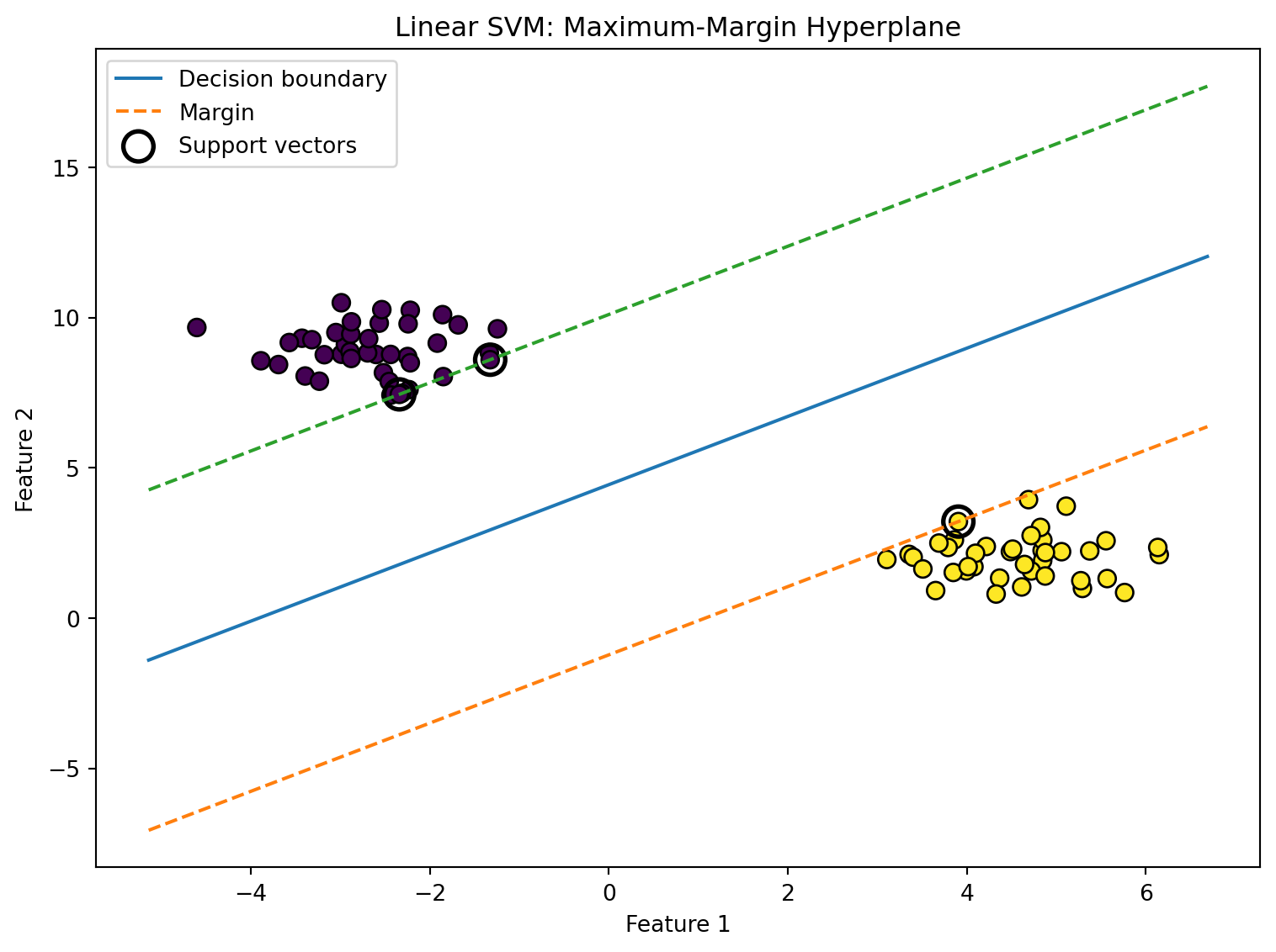
In the separable case, SVM seeks a hyperplane with maximum geometric margin.

2.1. Canonical Scaling

Because the hyperplane is unchanged if \(w\) and \(b\) are multiplied by a positive constant, we can impose the normalization

\[ \min_i y_i(w^\top x_i + b) = 1 \]

Then the closest points satisfy

\[ y_i(w^\top x_i + b) = 1 \]

The two margin boundary hyperplanes are

\[ w^\top x + b = \pm 1 \]

The decision boundary is

\[ w^\top x + b = 0 \]

NoteTheorem 1: Margin Width of a Canonically Scaled SVM

For the hyperplanes \(w^\top x + b = \pm 1\), the distance between them is

\[ \frac{2}{||w||} \]

2.2. Hard-Margin Optimization Problem

Maximizing \(\frac{2}{||w||}\) is equivalent to minimizing \(\frac{1}{2}||w||^2\). Therefore, the hard-margin SVM solves

\[ \min_{w,b}\frac{1}{2}||w||^2 \qquad \text{subject to } y_i(w^\top x_i+b)\geq 1, \quad i=1,\dots, n \]

This is a convex quadratic optimization problem with linear inequality constraints.

3. Support Vectors

NoteDefinition: Support Vector

A training point \(x_i\) is a support vector if it lies on the margin boundary:

\[ y_i(w^\top x_i + b) = 1 \]

These are the point closest to the separating hyperplane. They determine the final classifier.

Point satisfying

\[ y_i(w^\top x_i + b) > 1 \]

are correctly classified and lie outside the margin. In the hard-margin case, these non-support-vector points do not directly affect the final decision boundary once the support vectors are fixed.

This is one of the most important conceptual differences between SVMs and many other models. Linear regression uses all observations in estimating the fitted line, while a hard-margin SVM boundary is determined only by the support vectors.

import numpy as np
import matplotlib.pyplot as plt
from sklearn.datasets import make_blobs
from sklearn.svm import SVC

# Create linearly separable data
X, y = make_blobs(
    n_samples=80,
    centers=2,
    cluster_std=0.8,
    random_state=42
)

# Convert labels from {0,1} to {-1,+1} for conceptual consistency
y_signed = np.where(y == 0, -1, 1)

# Fit linear SVM with large C to approximate hard margin
clf = SVC(kernel="linear", C=1e6)
clf.fit(X, y_signed)

w = clf.coef_[0]
b = clf.intercept_[0]

# Plot data
plt.figure(figsize=(8, 6))
plt.scatter(X[:, 0], X[:, 1], c=y_signed, edgecolor="k", s=60)

# Plot decision boundary and margins
ax = plt.gca()
xlim = ax.get_xlim()
xx = np.linspace(xlim[0], xlim[1], 200)

# Decision boundary: w0*x + w1*y + b = 0
decision_boundary = -(w[0] * xx + b) / w[1]

# Margin boundaries: w0*x + w1*y + b = +/- 1
margin_positive = -(w[0] * xx + b - 1) / w[1]
margin_negative = -(w[0] * xx + b + 1) / w[1]

plt.plot(xx, decision_boundary, label="Decision boundary")
plt.plot(xx, margin_positive, linestyle="--", label="Margin")
plt.plot(xx, margin_negative, linestyle="--")

# Highlight support vectors
plt.scatter(
    clf.support_vectors_[:, 0],
    clf.support_vectors_[:, 1],
    s=180,
    facecolors="none",
    edgecolors="k",
    linewidths=2,
    label="Support vectors"
)

plt.title("Linear SVM: Maximum-Margin Hyperplane")
plt.xlabel("Feature 1")
plt.ylabel("Feature 2")
plt.legend()
plt.tight_layout()
plt.show()

print("w:", w)
print("b:", b)
print("Number of support vectors:", len(clf.support_vectors_))

Figure 1: Maximum-Margin Hyperplane

w: [ 0.20049367 -0.17658289]
b: 0.7845610916293154
Number of support vectors: 3

5. Lagrangian and KKT Conditions

5.1. Lagrangian and Dual Formulation

The dual formulation is central to SVMs because it allows the kernel trick. Recall, the hard-margin primal problem is

\[ \min_{w,b}\frac{1}{2}||w||^2 \qquad \text{subject to } y_i(w^\top x_i+b)\geq 1, \quad i=1,\dots, n \]

Equivalently,

\[ 1- y_i(w^\top x_i + b)\leq 0 \]

Introduce Lagrange multipliers \(\lambda_i\geq 0\). Then the Lagrangian is

\[ \begin{aligned} \mathcal L (w, b, \lambda) &= \frac{1}{2}||w||^2 + \sum_{i=1}^n\lambda_i[1-y_i(w^\top x_i+b)]\\ &=\frac{1}{2}w^\top w + \sum_{i=1}^n \lambda_i - \sum_{i=1}^n\lambda_iy_iw^\top x_i -b\sum_{i=1}^n \lambda_i y_i \end{aligned} \]

Now we calculate the gradient:

\[ \begin{aligned} \nabla_{w, b, \lambda}\mathcal L (w, b, \lambda)&=\left(\frac{\partial \mathcal L}{\partial w},\frac{\partial \mathcal L}{\partial b},\frac{\partial \mathcal L}{\partial \lambda}\right)\\ &=\left(w-\sum_{i=1}^n\lambda_i y_ix_i, -\sum_{i=1}^n \lambda_i y_i ,n-\sum_{i=1}^ny_i(w^\top x_i+b)\right) \end{aligned} \]

and therefore:

\[ \nabla_{w,b,\lambda}\mathcal L(w, b, \lambda)= 0\Longleftrightarrow \begin{cases} w=\sum_{i=1}^n \lambda_iy_ix_i\\ \sum_{i=1}^n \lambda_iy_i=0\\ n= \sum_{i=1}^ny_i(w^\top x_i+b) \end{cases} \]

We substitute back to the Lagrangian; the dual problem becomes¹:

\[ \begin{aligned} \max_\lambda \min_{w,b} \mathcal L(w,b, \lambda) &\sim \max_\lambda \sum_{i=1}^n \lambda_i -\frac{1}{2}\sum_{i=1}^n\sum_{j=1}^n \lambda_i \lambda_jy_iy_jx^\top_ix_j\\ \text{subject to }& \lambda_i\geq 0, \, i=1,\dots, n \\&\sum_{i=1}^n \lambda_iy_i =0 \end{aligned} \]

The decision function becomes

\[ f(x)=w^\top x+ b = \sum_{i=1}^n \lambda_iy_ix_i^\top x + b \] Only points with \(\lambda_i>0\) contribute to the decision function. These are the support vectors.

5.2. KTT Conditions

The Karush-Kuhn-Tucker, or KTT, conditions characterize the optimal solution of the constrained convex optimization problem.

For hard-margin SVM, the KKT conditions include:

1. Primal feasibility: \(y_i(w^\top x_i + b) \geq 1\).
2. Dual feasibility: \(\lambda_i \geq 0\).
3. Stationarity: \(w= \sum_{i=1}^n \lambda_i y_i x_i,\qquad \sum_{i=1}^n \lambda_iy_i = 0.\)
4. Complementary slackness: \(\lambda_i [y_i(w^\top x_i+b)-1]=0.\) Complementary slackness implies:
   • If \(y_i(w^\top x_i + b)> 1\) then \(\lambda_i = 0\).
   • If \(\lambda_i > 0\), then \(y_i (w^\top x_i + b)=1\).

Thus, only margin points have positive dual coefficients.

6. Soft-Margin SVM

Real-world data are often not linearly separable. Classes may overlap, labels may contain noise, or the true boundary may be nonlinear. A hard-margin SVM would fail if no separating hyperplane exists.

Soft-margin SVM introduces slack variables \(\xi_i\geq 0\) to allow margin violations. The constraints become

\[ y_i (w^\top x_i + b) \geq 1 - \xi_i. \]

The soft-margin primal problem is

\[ \begin{aligned} \min_{w, b, \xi} \frac{1}{2}||w||^2 + C\sum_{i=1}^n \xi_i\qquad \text{subject to }& y_i(w^\top x_i+b)\geq 1-\xi_i,\\ & \xi_i\geq 0 \end{aligned} \]

Here \(C>0\) is the regularization parameter.

6.1. Slack Variables

The slack variables \(\xi_i\) measures the violation of the margin constraint.

For an observation \(i\):

1. If \(\xi_i=0\), then \(y_i(w^\top x_i + b) \geq 1\). The point is correctly classified and outside or on the margin.
2. If \(0<\xi_i<1\), then \(0<y_i(w^\top x_i + b)<1\). The point is correctly classified but inside the margin.
3. If \(\xi_i\geq 1\), then \(y_i(w^\top x_i + b)\leq 0\). The point is misclassified or lies on the decision boundary.

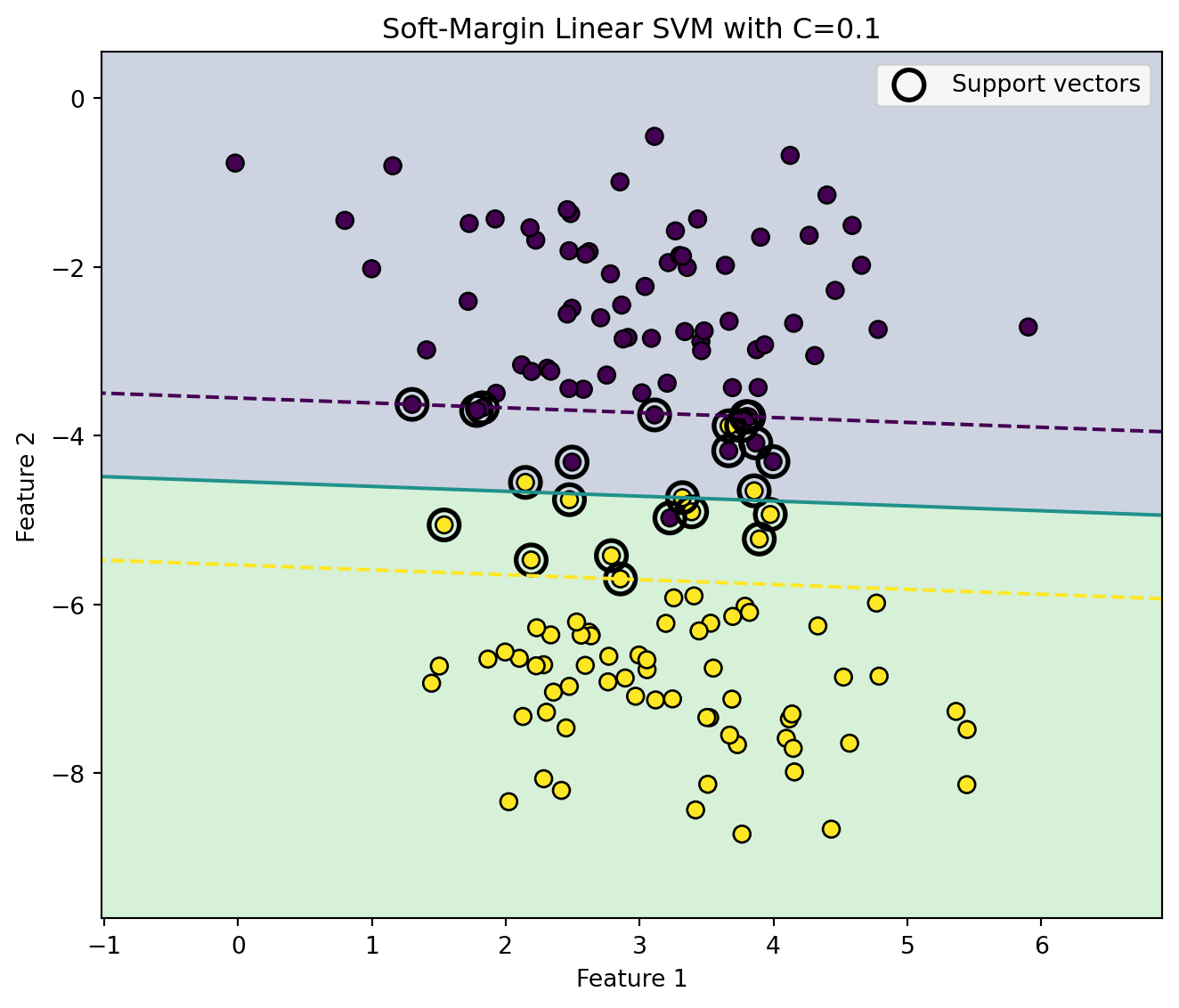
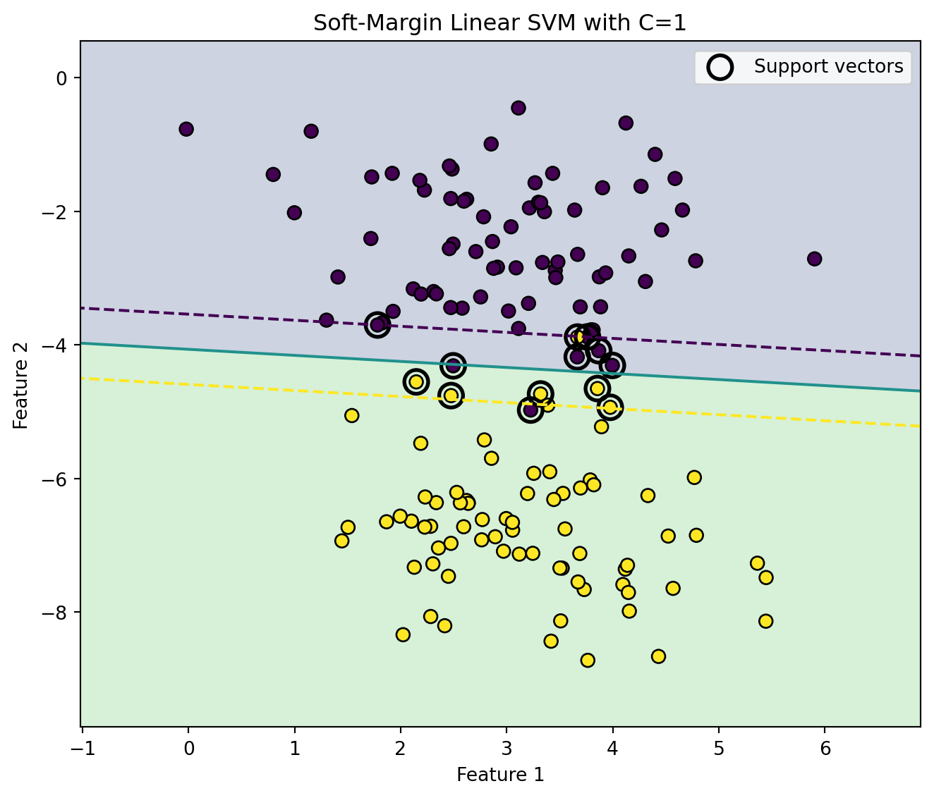
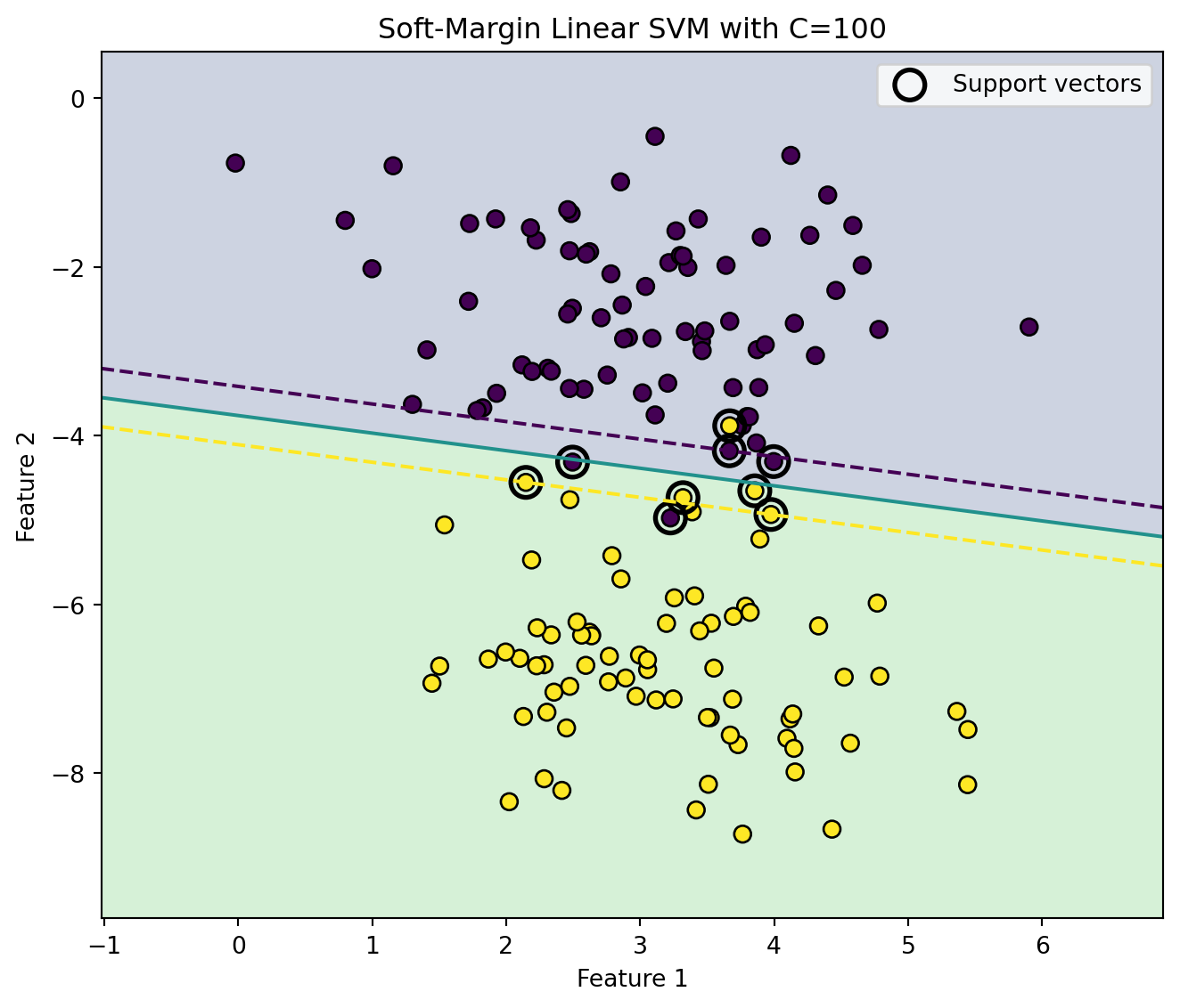
The parameter \(C\) controls the tradeoff between margin width and training violations.

• Large \(C\): violations are heavily penalized, so the model tries to classify training points correctly, potentially producing a smaller margin.
• Small \(C\): violations are tolerated, so the model prefers a wider margin and stronger regularization.

6.2. Hinge Loss Interpretation

The soft-margin SVM can also be written as unconstrained regularized empirical risk minimization using the hinge loss.

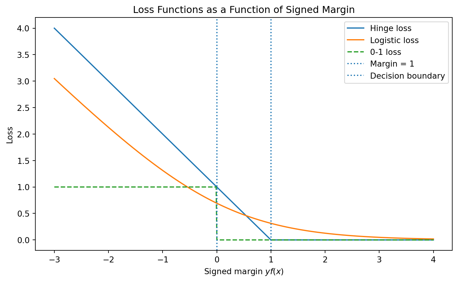
The hinge loss is

\[ L(y, f(x)) = \max(0, 1-yf(x)) \]

For a linear SVM \(f(x) = w^\top x+ b\). Then the primal objective can be written as

\[ \min_{w,b} \frac{1}{2} ||w||^2 + C\sum_{i=1}^n \max (0, 1-y_i(w^\top x_i + b)) \]

The hinge loss is zero when

\[ y_if(x_i) \geq 1. \]

It is positive when a point is inside the margin or misclassified.

This distinguishes SVM from logistic regression. Logistic regression uses log-loss,

\[ \log (1+\exp (-yf(x))) \]

which keeps penalizing all points, even those correctly classified with large margin. The hinge loss become zero once a point is correctly classified beyond the margin.

import numpy as np
import matplotlib.pyplot as plt

margin = np.linspace(-3, 4, 500)

hinge = np.maximum(0, 1 - margin)
logistic = np.log(1 + np.exp(-margin))
zero_one = (margin <= 0).astype(float)

plt.figure(figsize=(8, 5))
plt.plot(margin, hinge, label="Hinge loss")
plt.plot(margin, logistic, label="Logistic loss")
plt.plot(margin, zero_one, linestyle="--", label="0-1 loss")
plt.axvline(1, linestyle=":", label="Margin = 1")
plt.axvline(0, linestyle=":", label="Decision boundary")
plt.title("Loss Functions as a Function of Signed Margin")
plt.xlabel(r"Signed margin $y f(x)$")
plt.ylabel("Loss")
plt.legend()
plt.tight_layout()
plt.show()

Figure 2: Hinge Loss

6.3. Soft-Margin Dual Problem

For the soft-margin SVM, the dual problem becomes

\[ \begin{aligned} \max_\lambda \sum_{i=1}^n \lambda_i -\frac{1}{2}\sum_{i=1}^n\sum_{j=1}^n \lambda_i \lambda_jy_iy_jx^\top_ix_j\qquad \text{ subject to }& 0\leq\lambda_i\leq C, \, i=1,\dots, n \\&\sum_{i=1}^n \lambda_iy_i =0 \end{aligned} \]

Compared with the hard-margin dual, the only change is the upper bound \(\lambda_i\leq C\). This upper bound comes from the slack penalty. It limits how much influence any single training observation can have.

The decision function remains

\[ f(x)=w^\top x+ b = \sum_{i=1}^n \lambda_iy_ix_i^\top x + b \] In the soft-margin case, support vectors can include:

1. Points on the margin: \(0<\lambda_i<C\).
2. Points inside the margin or misclassified points: \(\lambda_i = C\).

The KKT conditions imply:

• If \(\lambda_i = 0\), the point is outside the margin and does not affect the boundary.
• If \(0<\lambda_i<C\), the point lies exactly on the margin.
• If \(\lambda_i =C\), the point is inside the margin or misclassified.

import numpy as np
import matplotlib.pyplot as plt
from sklearn.datasets import make_blobs
from sklearn.svm import SVC

X, y = make_blobs(
    n_samples=150,
    centers=2,
    cluster_std=1,
    random_state=30
)

y_signed = np.where(y == 0, -1, 1)

x_min, x_max = X[:, 0].min() - 1, X[:, 0].max() + 1
y_min, y_max = X[:, 1].min() - 1, X[:, 1].max() + 1

xx, yy = np.meshgrid(
    np.linspace(x_min, x_max, 400),
    np.linspace(y_min, y_max, 400)
)

grid = np.c_[xx.ravel(), yy.ravel()]

for C in [0.1, 1, 100]:
    clf = SVC(kernel="linear", C=C)
    clf.fit(X, y_signed)

    Z = clf.decision_function(grid).reshape(xx.shape)

    plt.figure(figsize=(7, 6))
    plt.contourf(xx, yy, Z > 0, alpha=0.25)
    plt.contour(xx, yy, Z, levels=[-1, 0, 1], linestyles=["--", "-", "--"])
    plt.scatter(X[:, 0], X[:, 1], c=y_signed, edgecolor="k", s=50)
    plt.scatter(
        clf.support_vectors_[:, 0],
        clf.support_vectors_[:, 1],
        s=160,
        facecolors="none",
        edgecolors="k",
        linewidths=2,
        label="Support vectors"
    )
    plt.title(f"Soft-Margin Linear SVM with C={C}")
    plt.xlabel("Feature 1")
    plt.ylabel("Feature 2")
    plt.legend()
    plt.tight_layout()
    plt.show()

7. Kernels and Nonlinear SVMs

7.1. Why Kernels?

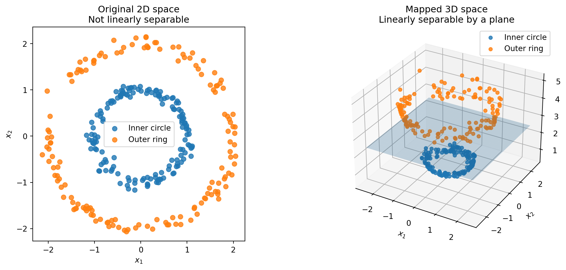
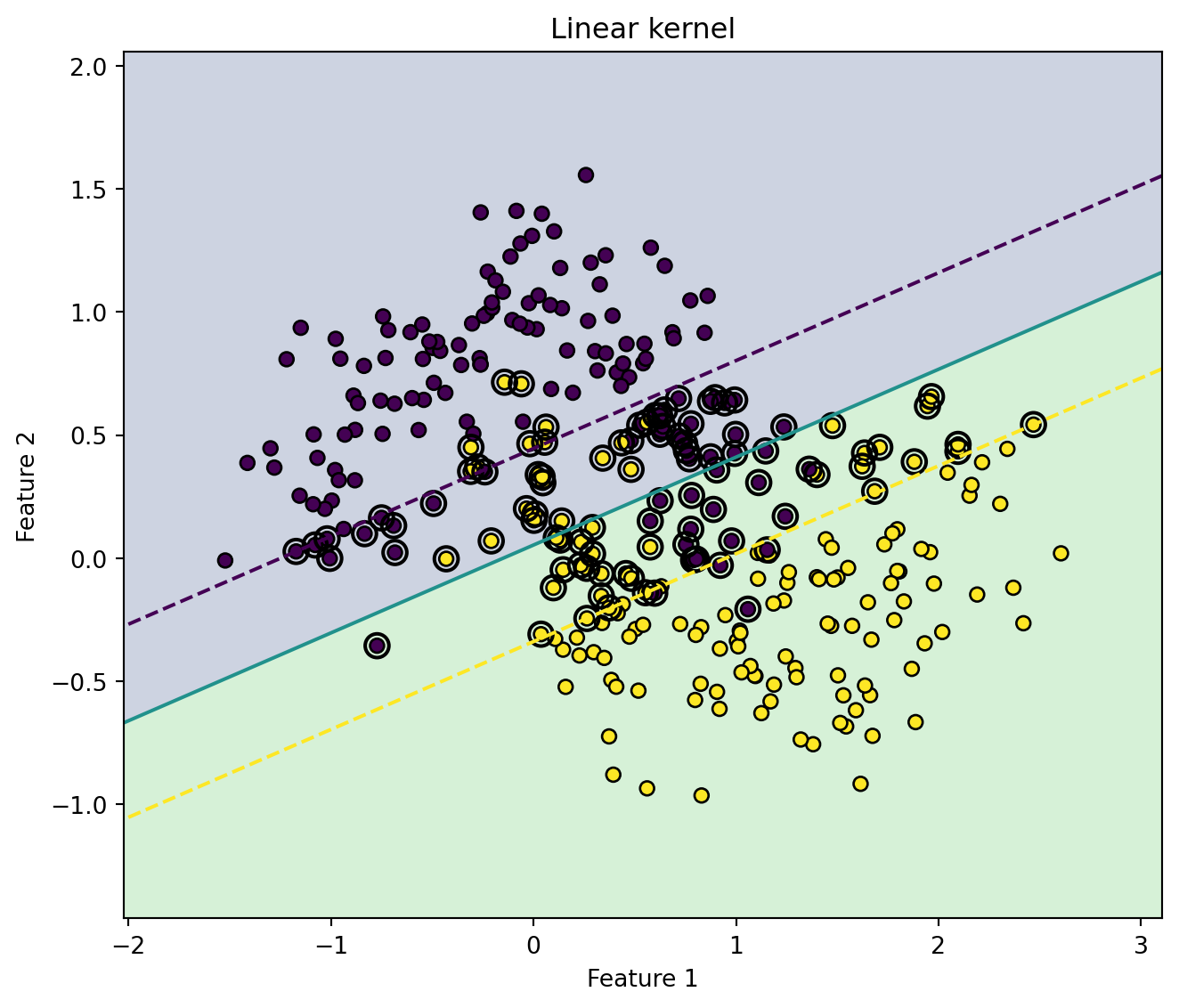
A linear SVM can only produce a linear decision boundary in the original feature space. But many classification problems are not linearly separable.

Suppose data in \(\mathbb R^2\) form concentric circles. No straight line can separate the inner circle from the outer ring. However, if we map the data into a higher-dimensional space, a linear separator may become possible.

import numpy as np
import matplotlib.pyplot as plt

np.random.seed(42)

n = 150

theta_inner = 2 * np.pi * np.random.rand(n)
theta_outer = 2 * np.pi * np.random.rand(n)

r_inner = 1.0 + 0.08 * np.random.randn(n)
r_outer = 2.0 + 0.08 * np.random.randn(n)

x_inner = r_inner * np.cos(theta_inner)
y_inner = r_inner * np.sin(theta_inner)

x_outer = r_outer * np.cos(theta_outer)
y_outer = r_outer * np.sin(theta_outer)

# Labels
label_inner = np.zeros(n)
label_outer = np.ones(n)

# Combine data
X2 = np.vstack([
    np.column_stack([x_inner, y_inner]),
    np.column_stack([x_outer, y_outer])
])

y = np.concatenate([label_inner, label_outer])

z_inner = x_inner**2 + y_inner**2
z_outer = x_outer**2 + y_outer**2

# Separating plane: z = constant
z_plane = 2.5

fig = plt.figure(figsize=(12, 5))

ax1 = fig.add_subplot(1, 2, 1)

ax1.scatter(x_inner, y_inner, label="Inner circle", alpha=0.8)
ax1.scatter(x_outer, y_outer, label="Outer ring", alpha=0.8)

ax1.set_title("Original 2D space\nNot linearly separable")
ax1.set_xlabel("$x_1$")
ax1.set_ylabel("$x_2$")
ax1.set_aspect("equal")
ax1.legend()

ax2 = fig.add_subplot(1, 2, 2, projection="3d")

ax2.scatter(x_inner, y_inner, z_inner, label="Inner circle", alpha=0.8)
ax2.scatter(x_outer, y_outer, z_outer, label="Outer ring", alpha=0.8)

# Draw separating plane z = 2.5
xx, yy = np.meshgrid(
    np.linspace(-2.5, 2.5, 20),
    np.linspace(-2.5, 2.5, 20)
)
zz = z_plane * np.ones_like(xx)

ax2.plot_surface(xx, yy, zz, alpha=0.25)

ax2.set_title("Mapped 3D space\nLinearly separable by a plane")
ax2.set_xlabel("$x_1$")
ax2.set_ylabel("$x_2$")
ax2.set_zlabel("$x_1^2 + x_2^2$")
ax2.legend()

plt.tight_layout()
plt.show()

Let \(\phi:\mathcal X \to \mathcal H\) be a feature map from the input space into a possibly high-dimensional feature space \(\mathcal H\). A linear SVM in feature space uses

\[ f(x) = w^\top \phi(x) + b. \]

The dual depends only on inner products:

\[ \phi(x_i)^\top \phi(x_j) \]

A kernel function computes this inner product directly:

$$ K(x_i,x_j) =
(x_i),(x_j).

$$

This is the kernel trick.

7.2. Kernelized Dual Problem

Replace \(x_i^\top x_j\) with \(K(x_i, x_j)\), we obtain the kernelized soft-margin dual:

\[ \begin{aligned} \max_\lambda \sum_{i=1}^n\lambda_i - \frac{1}{2}\sum_{i=1}^n\sum_{j=1}^n \lambda_i\lambda_jy_i y_j K(x_i, x_j) \qquad \text{subject to }& 0\leq \lambda_i\leq C,\\ & \sum_{i=1}^n\lambda_iy_i = 0. \end{aligned} \]

The decision function is

\[ f(x) = \sum_{i=1}^n \lambda_i y_iK(x_i, x) + b \]

Only support vectors with \(\lambda_i>0\) appear in the final sum.

NoteTheorem: Representer Theorem

For a broad class of regularized empirical risk minimization problems in a reproducing kernel Hilbert space, the minimizer has the form:

\[ f^*(x) = \sum_{i=1}^n \lambda_i K(x_i, x) \]

For SVM classification, because labels appear in the dual representation, the decision function can be written as:

\[ f(x) = \sum_{i=1}^n \lambda_i y_i K(x_i, x) + b \]

Even if the feature space is infinite-dimensional, the optimal solution lies in the span of kernel evaluations at the training point. This makes kernel methods computationally possible.

7.3. Common Kernel Functions

7.3.1. Linear Kernel

\[ K(x, z) = x^\top z \]

This gives the ordinary linear SVM.

Use the linear kernel when:

• the number of feature is large,
• the data are approximately linear separable,
• interpretability and speed matter,
• text features are sparse and high-dimensional.

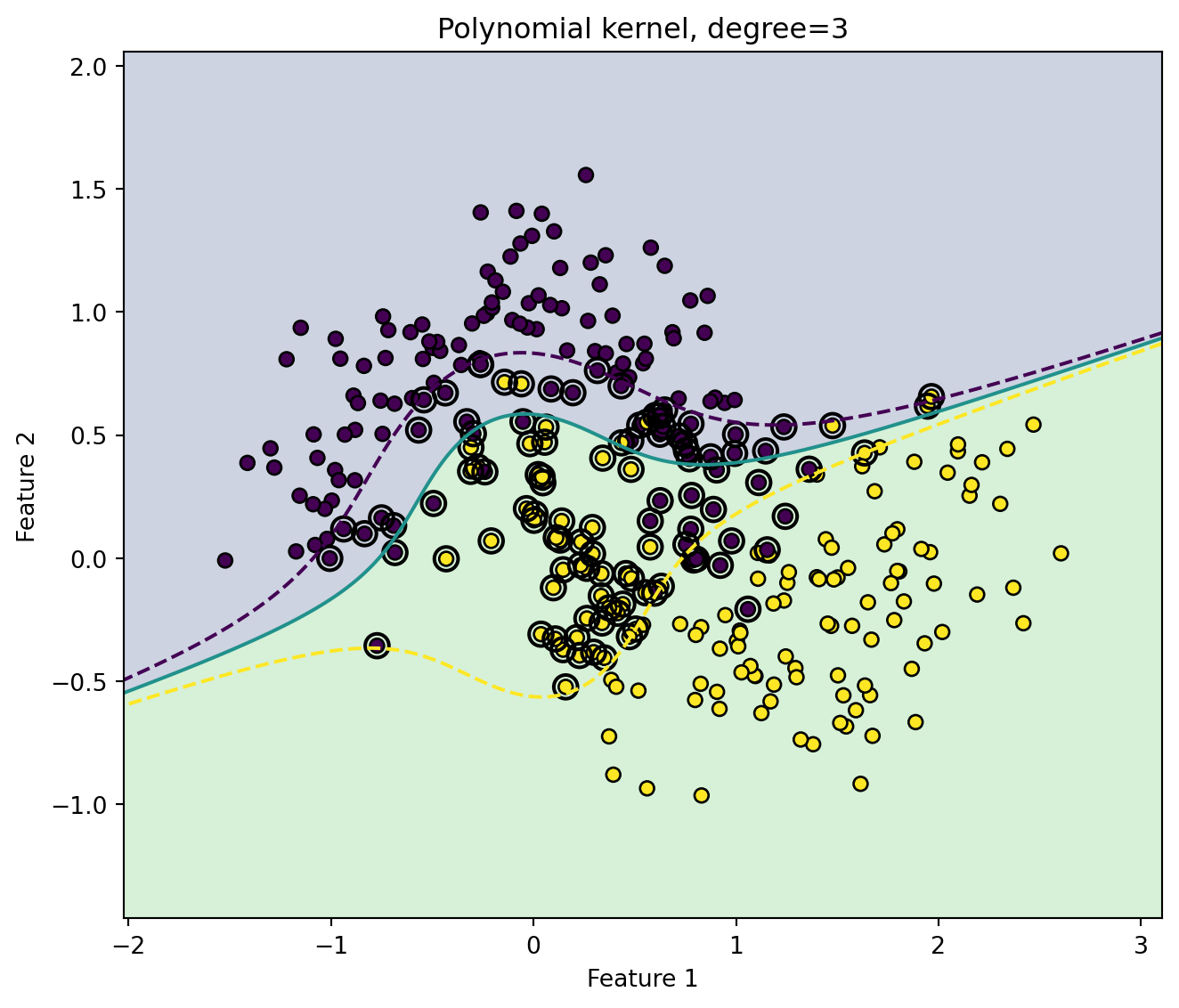
7.3.2. Polynomial Kernel

\[ K(x, z) = (c+x^\top z)^d \]

Here:

• \(d\) is the polynomial degree,
• \(c\geq 0\) controls the influence of lower-order terms.

The polynomial kernel captures feature interactions up to degree \(d\). For example, with two variables \(x_1, x_2\), a degree-2 polynomial feature map includes terms such as \(x_1^2, x_2^2, x_1x_2\).

Thus, a linear hyperplane in the polynomial feature space corresponds to a nonlinear boundary in the original input space.

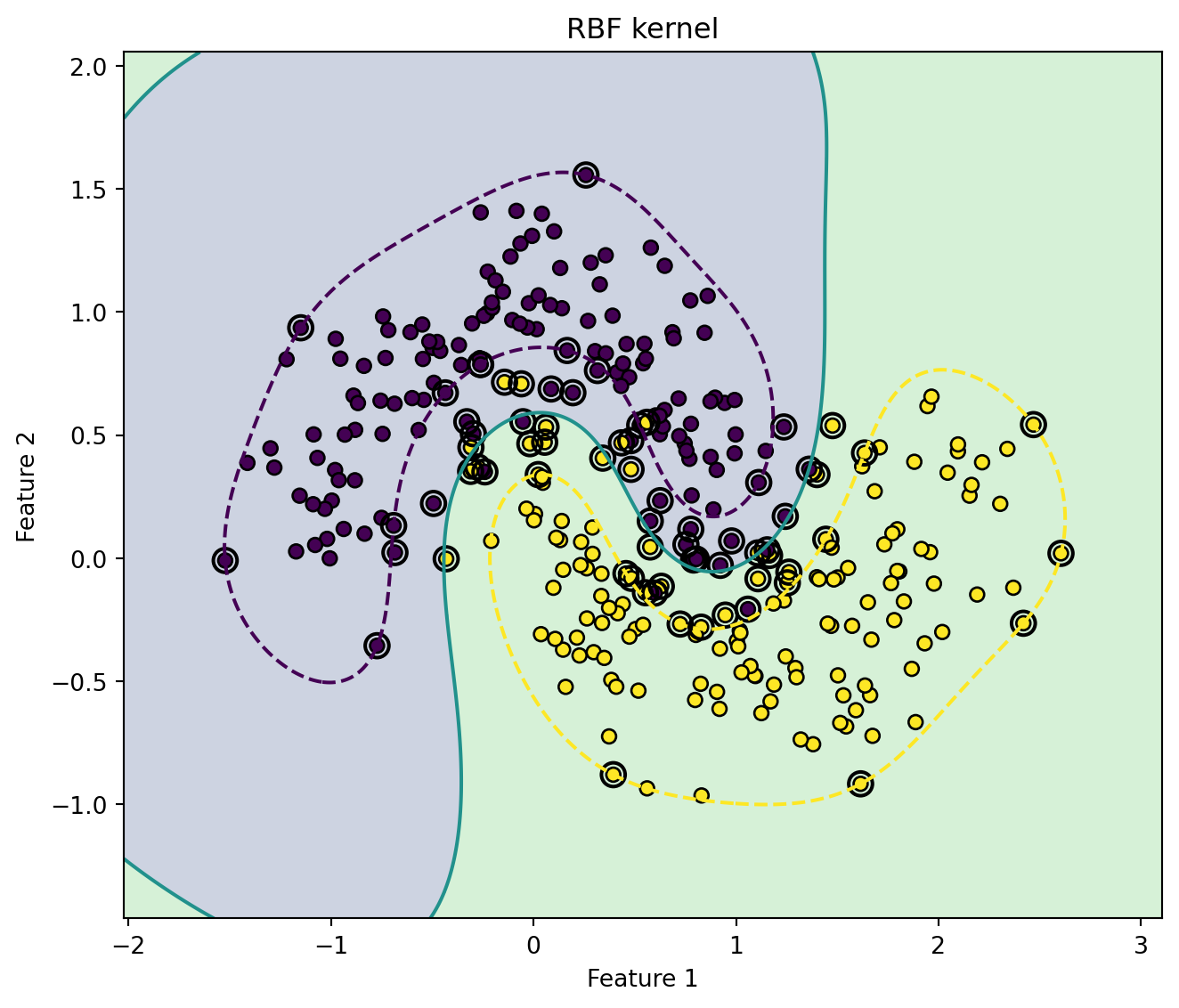
7.3.3. Gaussian Radial Basis Function Kernel

The Gaussian RBF kernel is

\[ K(x, z) = \exp(-\gamma ||x-z||^2), \]

where \(\gamma >0\). Equivalently,

\[ K (x, z) = \exp \left(-\frac{||x-z||^2}{2\sigma^2}\right), \]

where \(\gamma = \frac{1}{2\sigma^2}\).

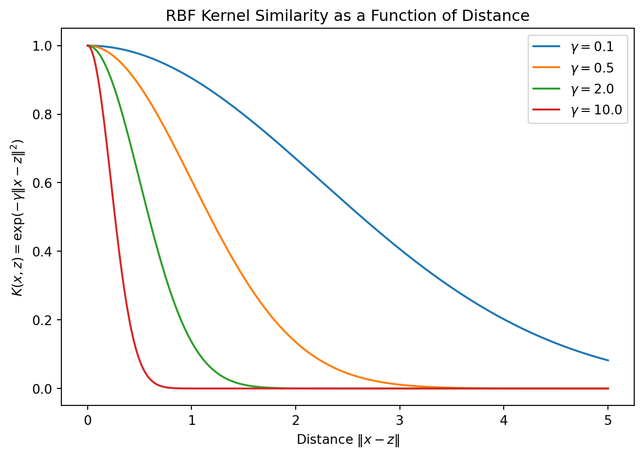
The RBF kernel creates local similarity: points close to each other have kernel value near 1, while far points have kernel value near 0.

The parameter \(\gamma\) controls the locality:

• small \(\gamma\): broad influence, smoother boundary.
• large \(\gamma\): local influence, more complex boundary.

import numpy as np
import matplotlib.pyplot as plt

distance = np.linspace(0, 5, 500)

for gamma in [0.1, 0.5, 2.0, 10.0]:
    similarity = np.exp(-gamma * distance**2)
    plt.plot(distance, similarity, label=fr"$\gamma={gamma}$")

plt.title("RBF Kernel Similarity as a Function of Distance")
plt.xlabel(r"Distance $\|x-z\|$")
plt.ylabel(r"$K(x,z)=\exp(-\gamma\|x-z\|^2)$")
plt.legend()
plt.tight_layout()
plt.show()

Figure 3: RBF Kernel as Local Similarity

7.3.4. Sigmoid Kernel

\[ K(x, z) = \tanh(\kappa_1x^\top z +\kappa_2) \]

The sigmoid kernel resembles the activation function used in neural networks. However, it is not positive semidefinite for all parameter values, so it must be used carefully.

7.3.5. Kernel Matrix

For training data \(x_1, \dots, x_n\), we define the kernel matrix \(K\in \mathbb R^{n\times n}\) by

\[ K_{ij} = K(x_i, x_j) \]

A valid kernel matrix must be:

• symmetric: \(K_{ij} = K_{ji}\),
• and positive semidefinite: \(c^\top K c\geq 0 \quad \forall c\in \mathbb R^n\).

This condition ensures that the kernel corresponds to an inner produce in some feature space.

import numpy as np
import matplotlib.pyplot as plt
from sklearn.datasets import make_moons
from sklearn.svm import SVC

X, y = make_moons(n_samples=300, noise=0.22, random_state=42)
y_signed = np.where(y == 0, -1, 1)

x_min, x_max = X[:, 0].min() - 0.5, X[:, 0].max() + 0.5
y_min, y_max = X[:, 1].min() - 0.5, X[:, 1].max() + 0.5

xx, yy = np.meshgrid(
    np.linspace(x_min, x_max, 400),
    np.linspace(y_min, y_max, 400)
)

grid = np.c_[xx.ravel(), yy.ravel()]

models = [
    ("Linear kernel", SVC(kernel="linear", C=1)),
    ("Polynomial kernel, degree=3", SVC(kernel="poly", degree=3, C=1, gamma="scale")),
    ("RBF kernel", SVC(kernel="rbf", C=1, gamma=2))
]

for title, clf in models:
    clf.fit(X, y_signed)
    Z = clf.decision_function(grid).reshape(xx.shape)

    plt.figure(figsize=(7, 6))
    plt.contourf(xx, yy, Z > 0, alpha=0.25)
    plt.contour(xx, yy, Z, levels=[-1, 0, 1], linestyles=["--", "-", "--"])
    plt.scatter(X[:, 0], X[:, 1], c=y_signed, edgecolor="k", s=35)
    plt.scatter(
        clf.support_vectors_[:, 0],
        clf.support_vectors_[:, 1],
        s=100,
        facecolors="none",
        edgecolors="k",
        linewidths=1.5
    )
    plt.title(title)
    plt.xlabel("Feature 1")
    plt.ylabel("Feature 2")
    plt.tight_layout()
    plt.show()

(a) Kernel Decision Boundaries

(b)

(c)

Figure 4

8. SVM Regression

8.1. Support Vector Regression

Support Vector Regression, or SVR, extends the maximum-margin idea to continuous targets.

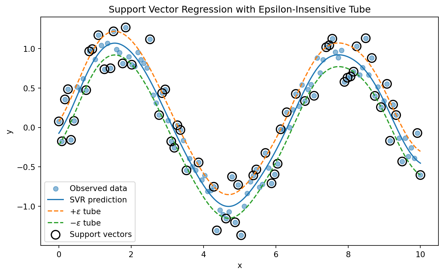
In ordinary regression, the goal is often to minimize squared error \((y_i-f(x_i))^2\). SVR instead uses an \(\epsilon\)-insensitive loss function. Errors smaller than \(\epsilon\) are ignored.

NoteDefinition: \(\epsilon\)-Insensitive Loss

The \(\epsilon\)-insensitive loss is:

\[ L_\epsilon(y, f(x)) = \max (0, |y-f(x)|-\epsilon). \]

If \(|y-f(x)|\leq \epsilon_i\), then \(L_\epsilon(y, f(x))=0\). Thus, predictions inside the \(\epsilon\)-tube receive no penalty.

8.2. Primal Form of Linear SVR

For linear SVR,

\[ f(x) = w^\top x+ b \]

Introduce slack variables \(\xi_i, xi_i^*\geq 0\). The primal SVR problem is

\[ \begin{aligned} \min_{w, b, \xi, \xi^*} \frac{1}{2} \|w\|^2 + C\sum_{i=1}^n(\xi_i + \xi_i^*)\quad \text{subject to } & y_i -(w^\top x_i + b) \leq \epsilon + \xi_i,\\ & (w^\top x_i + b) - y_i \leq \epsilon + \xi_i^*,\\ &\xi_i, \xi_i^*\geq 0. \end{aligned} \]

The first constraint handles observations above the tube. The second handles observations below the tube.

SVR is sparse because only points outside or on the boundary of the \(\epsilon\)-tube contribute to the solution. Points strictly inside the tube do not influence the fitted function.

import numpy as np
import matplotlib.pyplot as plt
from sklearn.svm import SVR

rng = np.random.default_rng(42)

X = np.linspace(0, 10, 120).reshape(-1, 1)
y = np.sin(X).ravel() + 0.25 * rng.normal(size=X.shape[0])

svr = SVR(kernel="rbf", C=10, gamma=0.5, epsilon=0.15)
svr.fit(X, y)

X_grid = np.linspace(0, 10, 500).reshape(-1, 1)
y_pred = svr.predict(X_grid)

epsilon = svr.epsilon

plt.figure(figsize=(8, 5))
plt.scatter(X, y, alpha=0.5, label="Observed data")
plt.plot(X_grid, y_pred, label="SVR prediction")
plt.plot(X_grid, y_pred + epsilon, linestyle="--", label=r"$+\epsilon$ tube")
plt.plot(X_grid, y_pred - epsilon, linestyle="--", label=r"$-\epsilon$ tube")

plt.scatter(
    X[svr.support_],
    y[svr.support_],
    s=120,
    facecolors="none",
    edgecolors="k",
    linewidths=1.5,
    label="Support vectors"
)

plt.title("Support Vector Regression with Epsilon-Insensitive Tube")
plt.xlabel("x")
plt.ylabel("y")
plt.legend()
plt.tight_layout()
plt.show()

print("Number of support vectors:", len(svr.support_))

Figure 5: SVR with epsilon-Tube

Number of support vectors: 63

9. SVM Extensions

9.1. Multiclass SVM

The standard SVM formulation is binary. For multiclass problems \(Y\in \{1, 2,\dots, K\}\), binary SVMs can be combined in several ways.

9.1.1. One-versus-Rest

One-versus-rest trains \(K\) binary classifiers. For class \(k\), we define labels

\[ y_i^{(k)}=\begin{cases} +1,& y_i = k\\ -1, & y_i\neq k \end{cases} \]

We then train one SVM per class \(f_k(x)\). Finally, we predict

\[ \hat y(x) = \arg\max_k f_k(x) \]

9.1.2. One-versus-One

One-versus-one trains a binary SVM for every pair of classes. The number of classifiers is

\[ \frac{K(K-1)}{2} \]

Each classifier votes for one class. The final predicition is the class with the most votes.

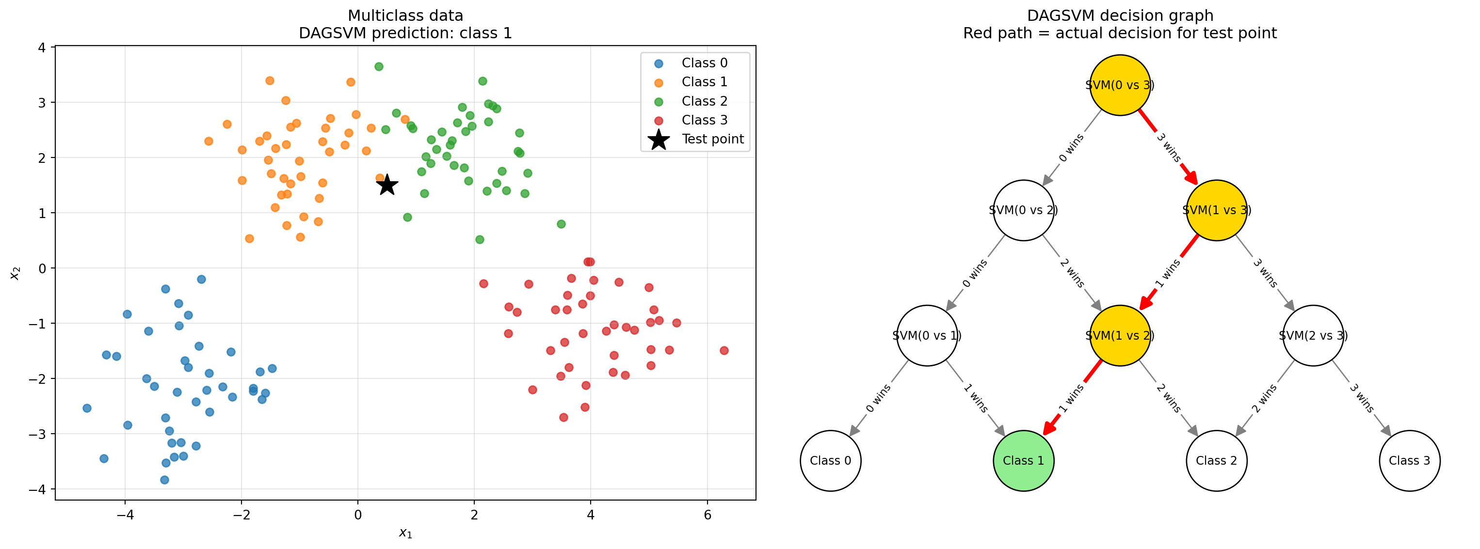
9.1.3. Directed Acyclic Graph SVM

DAGSVM organizes pairwise classifier into a directed acyclic graph. At each node, one class is eliminated until only one class remains.

import numpy as np
import matplotlib.pyplot as plt
import networkx as nx

from itertools import combinations
from sklearn.datasets import make_blobs
from sklearn.svm import SVC

X, y = make_blobs(
    n_samples=160,
    centers=[[-3, -2], [-1, 2], [2, 2], [4, -1]],
    cluster_std=0.8,
    random_state=7
)

classes = np.unique(y)
K = len(classes)

pairwise_svms = {}

for c1, c2 in combinations(classes, 2):
    mask = (y == c1) | (y == c2)

    clf = SVC(kernel="linear", C=10)
    clf.fit(X[mask], y[mask])

    pairwise_svms[(c1, c2)] = clf
    
def pair_node(i, j):
    return f"SVM({classes[i]} vs {classes[j]})"

def class_node(c):
    return f"Class {c}"

def dagsvm_predict_one(x):
    """
    DAGSVM decision rule:
    Start with class index i = 0 and j = K-1.
    At each node, compare classes[i] vs classes[j].
    The loser is eliminated.
    """
    i = 0
    j = K - 1

    path_text = []
    path_edges = []

    while i < j:
        c_left = classes[i]
        c_right = classes[j]

        clf = pairwise_svms[(c_left, c_right)]
        winner = clf.predict(x.reshape(1, -1))[0]

        current_node = pair_node(i, j)

        if winner == c_left:
            # c_left wins, so eliminate c_right
            eliminated = c_right

            if i < j - 1:
                next_node = pair_node(i, j - 1)
            else:
                next_node = class_node(c_left)

            path_text.append(
                f"{current_node}: class {c_left} wins, eliminate class {eliminated}"
            )
            path_edges.append((current_node, next_node))

            j -= 1

        else:
            # c_right wins, so eliminate c_left
            eliminated = c_left

            if i + 1 < j:
                next_node = pair_node(i + 1, j)
            else:
                next_node = class_node(c_right)

            path_text.append(
                f"{current_node}: class {c_right} wins, eliminate class {eliminated}"
            )
            path_edges.append((current_node, next_node))

            i += 1

    final_class = classes[i]
    return final_class, path_text, path_edges
    

x_test = np.array([0.5, 1.5])

pred_class, path_text, path_edges = dagsvm_predict_one(x_test)

print("DAGSVM decision path:")
for step in path_text:
    print(step)

print("\nFinal predicted class:", pred_class)

DAGSVM decision path:
SVM(0 vs 3): class 3 wins, eliminate class 0
SVM(1 vs 3): class 1 wins, eliminate class 3
SVM(1 vs 2): class 1 wins, eliminate class 2

Final predicted class: 1

G = nx.DiGraph()

# Add pairwise SVM nodes
for i in range(K):
    for j in range(i + 1, K):
        G.add_node(pair_node(i, j))

# Add terminal class nodes
for c in classes:
    G.add_node(class_node(c))

# Add DAG edges
for i in range(K):
    for j in range(i + 1, K):
        current = pair_node(i, j)

        # If left class wins, eliminate right class
        if i < j - 1:
            next_left_win = pair_node(i, j - 1)
        else:
            next_left_win = class_node(classes[i])

        # If right class wins, eliminate left class
        if i + 1 < j:
            next_right_win = pair_node(i + 1, j)
        else:
            next_right_win = class_node(classes[j])

        G.add_edge(current, next_left_win, label=f"{classes[i]} wins")
        G.add_edge(current, next_right_win, label=f"{classes[j]} wins")
        
fig, axes = plt.subplots(1, 2, figsize=(16, 6))

ax = axes[0]

for c in classes:
    ax.scatter(
        X[y == c, 0],
        X[y == c, 1],
        label=f"Class {c}",
        alpha=0.75
    )

ax.scatter(
    x_test[0],
    x_test[1],
    marker="*",
    s=300,
    color="black",
    label="Test point"
)

ax.set_title(f"Multiclass data\nDAGSVM prediction: class {pred_class}")
ax.set_xlabel("$x_1$")
ax.set_ylabel("$x_2$")
ax.legend()
ax.grid(alpha=0.3)

ax = axes[1]

# Manual triangular layout
pos = {}

for i in range(K):
    for j in range(i + 1, K):
        pos[pair_node(i, j)] = ((i + j) / 2, j - i)

for i, c in enumerate(classes):
    pos[class_node(c)] = (i, 0)

path_edges_set = set(path_edges)
path_nodes = set()

for u, v in path_edges:
    path_nodes.add(u)
    path_nodes.add(v)

node_colors = []
for node in G.nodes():
    if node == class_node(pred_class):
        node_colors.append("lightgreen")
    elif node in path_nodes:
        node_colors.append("gold")
    else:
        node_colors.append("white")

edge_colors = []
edge_widths = []

for edge in G.edges():
    if edge in path_edges_set:
        edge_colors.append("red")
        edge_widths.append(3.0)
    else:
        edge_colors.append("gray")
        edge_widths.append(1.0)

nx.draw(
    G,
    pos,
    ax=ax,
    with_labels=True,
    node_color=node_colors,
    edge_color=edge_colors,
    width=edge_widths,
    node_size=2200,
    font_size=9,
    arrows=True,
    arrowsize=18,
    edgecolors="black"
)

edge_labels = nx.get_edge_attributes(G, "label")

nx.draw_networkx_edge_labels(
    G,
    pos,
    edge_labels=edge_labels,
    ax=ax,
    font_size=8
)

ax.set_title("DAGSVM decision graph\nRed path = actual decision for test point")
ax.axis("off")

plt.tight_layout()
plt.show()

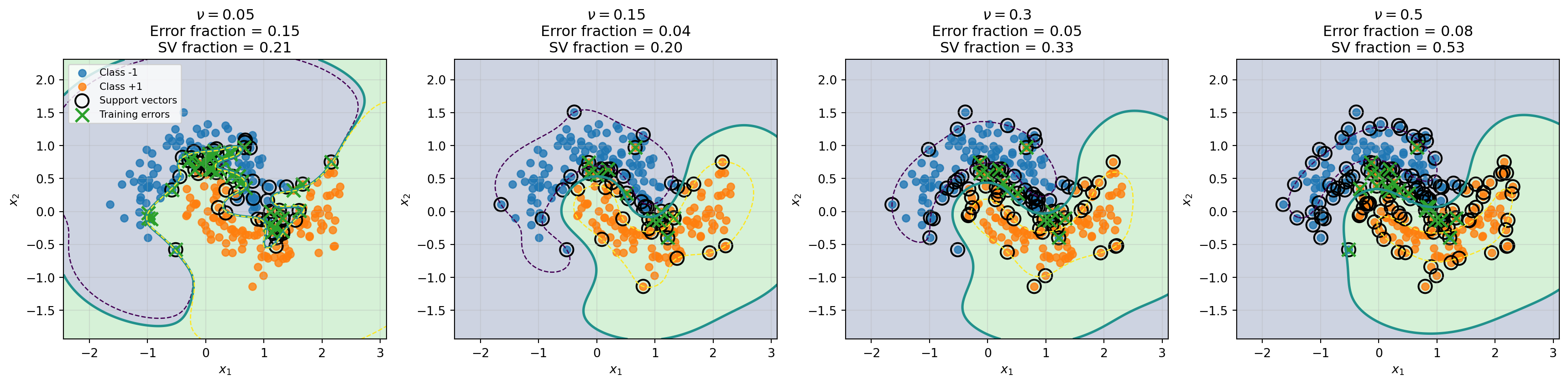
9.2. \(\nu\)-SVM

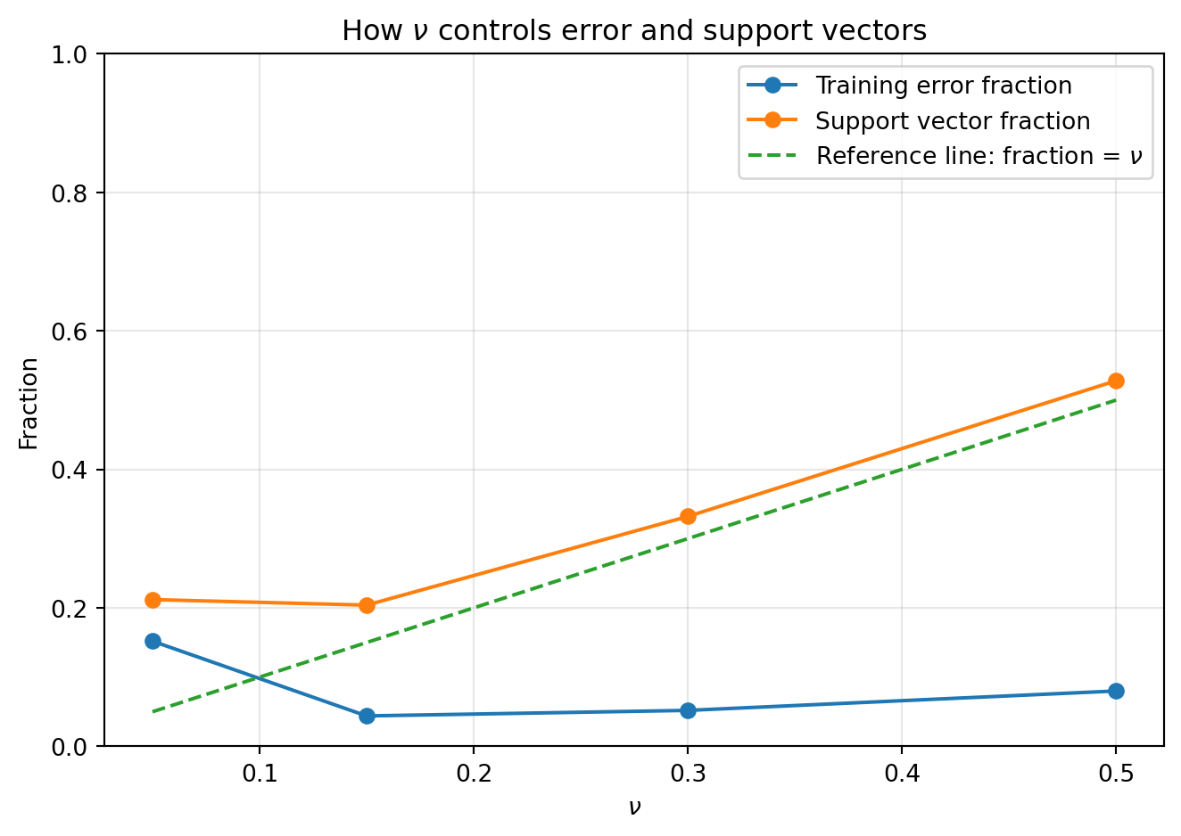
The \(\nu\)-SVM reformulates the regularization problem using a parameter \(\nu\in (0, 1]\). This parameter has an intuitive interpretation:

• \(\nu\) is an upper bound on the fraction of margin errors.
• \(\nu\) is a lower bound on the fraction of support vectors.

The exact interpretation depends on the formulation and conditions, but the main idea is that \(\nu\) gives direct control over the expected support vector and error behavior.

import numpy as np
import matplotlib.pyplot as plt

from sklearn.datasets import make_moons
from sklearn.preprocessing import StandardScaler
from sklearn.pipeline import make_pipeline
from sklearn.svm import NuSVC

X, y = make_moons(
    n_samples=250,
    noise=0.25,
    random_state=7
)

# Convert labels from {0, 1} to {-1, +1}
y_signed = np.where(y == 0, -1, 1)

nu_values = [0.05, 0.15, 0.30, 0.50]

models = []
results = []

for nu in nu_values:
    model = make_pipeline(
        StandardScaler(),
        NuSVC(kernel="rbf", gamma=1.0, nu=nu)
    )

    model.fit(X, y_signed)

    y_pred = model.predict(X)

    # Training error fraction
    error_fraction = np.mean(y_pred != y_signed)

    # Support vector fraction
    svc = model.named_steps["nusvc"]
    sv_fraction = len(svc.support_) / len(X)

    models.append(model)

    results.append({
        "nu": nu,
        "error_fraction": error_fraction,
        "sv_fraction": sv_fraction
    })

x_min, x_max = X[:, 0].min() - 0.8, X[:, 0].max() + 0.8
y_min, y_max = X[:, 1].min() - 0.8, X[:, 1].max() + 0.8

xx, yy = np.meshgrid(
    np.linspace(x_min, x_max, 400),
    np.linspace(y_min, y_max, 400)
)

grid = np.c_[xx.ravel(), yy.ravel()]

fig, axes = plt.subplots(1, len(nu_values), figsize=(18, 4.5))

for ax, nu, model, result in zip(axes, nu_values, models, results):
    Z = model.decision_function(grid).reshape(xx.shape)

    svc = model.named_steps["nusvc"]
    scaler = model.named_steps["standardscaler"]

    # Support vectors are stored in scaled space,
    # so convert them back to original space.
    support_vectors_original = scaler.inverse_transform(svc.support_vectors_)

    y_pred = model.predict(X)
    mistakes = y_pred != y_signed

    # Decision regions
    ax.contourf(xx, yy, Z > 0, alpha=0.25)

    # Decision boundary and margins
    ax.contour(
        xx,
        yy,
        Z,
        levels=[-1, 0, 1],
        linestyles=["--", "-", "--"],
        linewidths=[1, 2, 1]
    )

    # Training data
    ax.scatter(
        X[y_signed == -1, 0],
        X[y_signed == -1, 1],
        label="Class -1",
        alpha=0.8
    )

    ax.scatter(
        X[y_signed == 1, 0],
        X[y_signed == 1, 1],
        label="Class +1",
        alpha=0.8
    )

    # Support vectors
    ax.scatter(
        support_vectors_original[:, 0],
        support_vectors_original[:, 1],
        s=120,
        facecolors="none",
        edgecolors="black",
        linewidths=1.5,
        label="Support vectors"
    )

    # Misclassified points
    ax.scatter(
        X[mistakes, 0],
        X[mistakes, 1],
        marker="x",
        s=120,
        linewidths=2,
        label="Training errors"
    )

    ax.set_title(
        rf"$\nu={nu}$"
        + "\n"
        + f"Error fraction = {result['error_fraction']:.2f}"
        + "\n"
        + f"SV fraction = {result['sv_fraction']:.2f}"
    )

    ax.set_xlabel("$x_1$")
    ax.set_ylabel("$x_2$")
    ax.grid(alpha=0.3)

axes[0].legend(loc="upper left", fontsize=8)

plt.tight_layout()
plt.show()

nu_list = [r["nu"] for r in results]
err_list = [r["error_fraction"] for r in results]
sv_list = [r["sv_fraction"] for r in results]

plt.figure(figsize=(7, 5))

plt.plot(
    nu_list,
    err_list,
    marker="o",
    label="Training error fraction"
)

plt.plot(
    nu_list,
    sv_list,
    marker="o",
    label="Support vector fraction"
)

plt.plot(
    nu_list,
    nu_list,
    linestyle="--",
    label=r"Reference line: fraction = $\nu$"
)

plt.title(r"How $\nu$ controls error and support vectors")
plt.xlabel(r"$\nu$")
plt.ylabel("Fraction")
plt.ylim(0, 1)
plt.grid(alpha=0.3)
plt.legend()

plt.tight_layout()
plt.show()

9.3. One-Class SVM

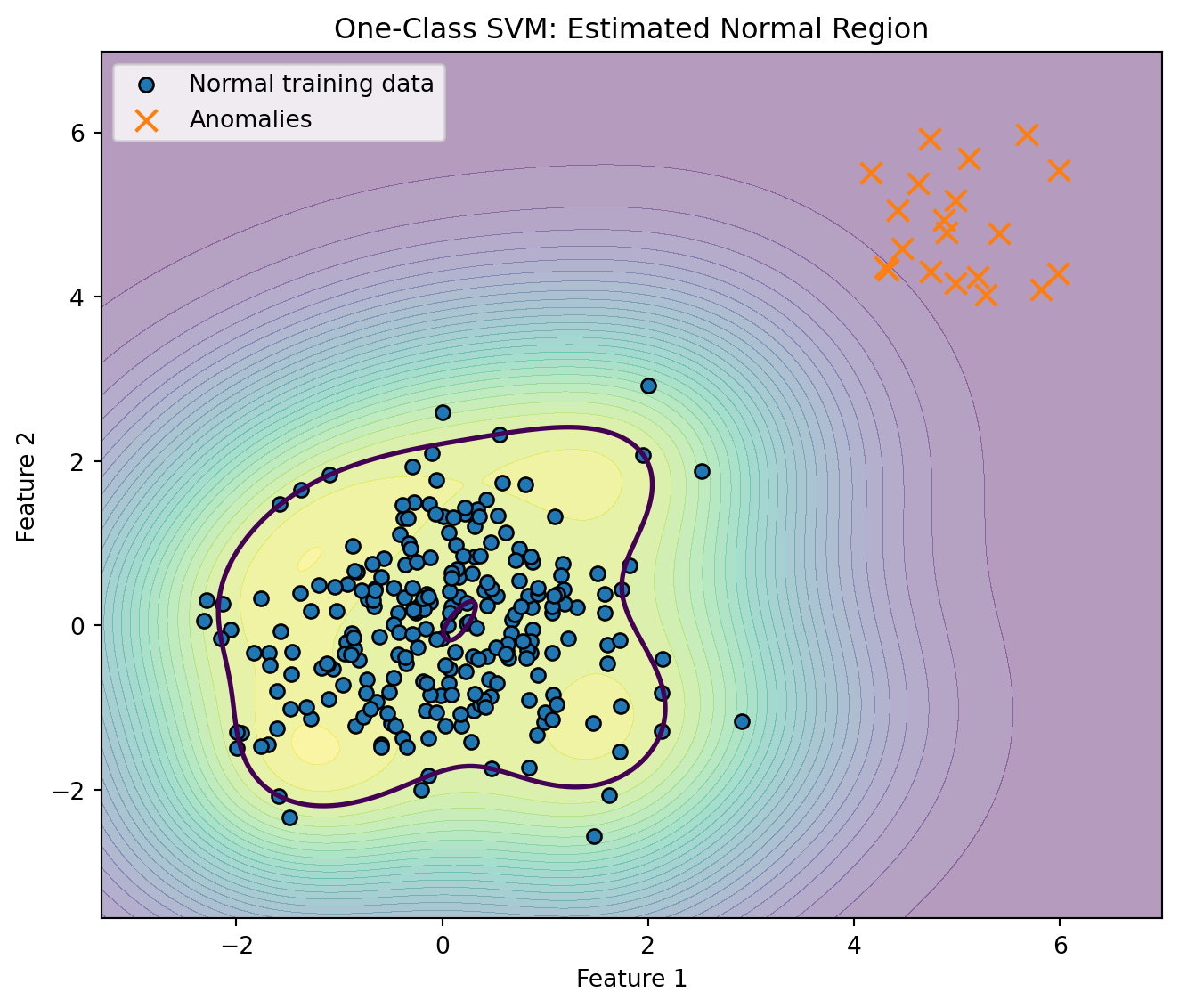
One-class SVM is used for novelty detection and anomaly detection. It is trained primarily on normal data and attempts to find a boundary enclosing the high-density region.

The one-class SVM solves a problem of the form

\[ \begin{aligned} \min_{w, \rho, \xi} \frac{1}{2} \|w\|^2 + \frac{1}{\nu n} \sum_{i=1}^n \xi_i -\rho\quad \text{subject to } & w^\top \phi(x_i)\geq \rho -\xi_i,\\ & \xi_i\geq 0. \end{aligned} \]

The decision function is

\[ f(x) = \text{sign}(w^\top \phi (x) - \rho). \]

Points with \(f(x)<0\) are treated as anomalies or outliers.

import numpy as np
import matplotlib.pyplot as plt
from sklearn.svm import OneClassSVM

rng = np.random.default_rng(42)

# Normal data
X_normal = rng.normal(loc=0, scale=1, size=(250, 2))

# Anomalies
X_anomaly = rng.uniform(low=4, high=6, size=(20, 2))

X = np.vstack([X_normal, X_anomaly])

ocsvm = OneClassSVM(kernel="rbf", gamma=0.4, nu=0.08)
ocsvm.fit(X_normal)

x_min, x_max = X[:, 0].min() - 1, X[:, 0].max() + 1
y_min, y_max = X[:, 1].min() - 1, X[:, 1].max() + 1

xx, yy = np.meshgrid(
    np.linspace(x_min, x_max, 400),
    np.linspace(y_min, y_max, 400)
)

grid = np.c_[xx.ravel(), yy.ravel()]
Z = ocsvm.decision_function(grid).reshape(xx.shape)

plt.figure(figsize=(7, 6))
plt.contourf(xx, yy, Z, levels=30, alpha=0.4)
plt.contour(xx, yy, Z, levels=[0], linewidths=2)
plt.scatter(X_normal[:, 0], X_normal[:, 1], edgecolor="k", label="Normal training data")
plt.scatter(X_anomaly[:, 0], X_anomaly[:, 1], marker="x", s=80, label="Anomalies")
plt.title("One-Class SVM: Estimated Normal Region")
plt.xlabel("Feature 1")
plt.ylabel("Feature 2")
plt.legend()
plt.tight_layout()
plt.show()

Figure 6: One-class SVM for Anomaly Detection

9.4. Least Squares SVM

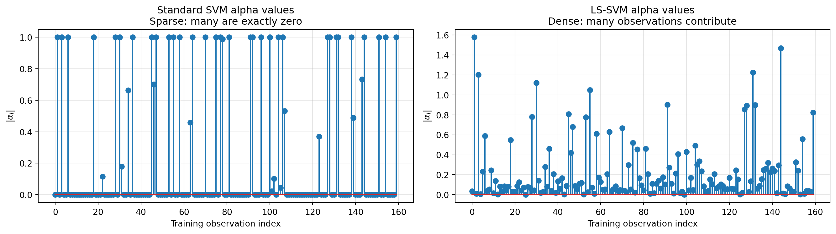
Least square SVM, or LS-SVM, modifies the classical SVM optimization problem by replacing inequality constraints with equality constraints and using squared errors.

A simplified LS-SVM classification formulation is

\[ \min_{w, b , e} \frac{1}{2} \|w\|^2 +\frac{\gamma}{2}\sum_{i=1}^n e_i^2 \quad \text{subject to } y_i(w^\top \phi (x_i)+b) = 1-e_i. \]

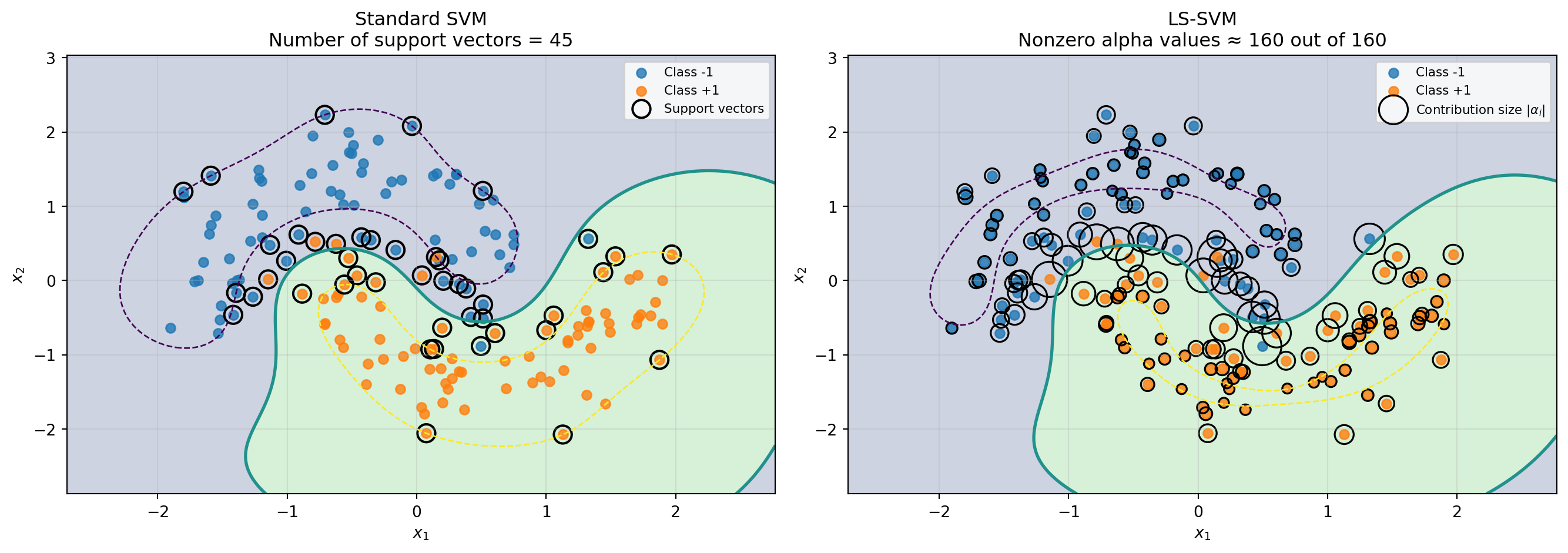
The classical SVM requires solving a quadratic programming problem with inequality constraints. LS-SVM leads to a system of linear equations, which can be computationally faster.

The tradeoff is that LS-SVM loses some of the sparsity of standard SVM, because squared loss usually makes more observations contribute to the solution.

import numpy as np
import matplotlib.pyplot as plt

from sklearn.datasets import make_moons
from sklearn.preprocessing import StandardScaler
from sklearn.svm import SVC
from sklearn.metrics.pairwise import rbf_kernel

X, y = make_moons(
    n_samples=160,
    noise=0.25,
    random_state=7
)

# Convert labels from {0, 1} to {-1, +1}
y_signed = np.where(y == 0, -1, 1)

# Standardize the data
scaler = StandardScaler()
X_scaled = scaler.fit_transform(X)

class LSSVM:
    def __init__(self, gamma=1.0, rbf_gamma=1.0):
        """
        gamma:
            LS-SVM regularization parameter.
            Larger gamma means errors are penalized more heavily.

        rbf_gamma:
            Kernel parameter for the RBF kernel.
        """
        self.gamma = gamma
        self.rbf_gamma = rbf_gamma

    def fit(self, X, y):
        self.X_train = X
        self.y_train = y.astype(float)

        n = X.shape[0]

        # Kernel matrix K(x_i, x_j)
        K = rbf_kernel(X, X, gamma=self.rbf_gamma)

        # Omega_ij = y_i y_j K(x_i, x_j)
        Omega = np.outer(self.y_train, self.y_train) * K

        # LS-SVM linear system:
        #
        # [ 0   y^T              ] [ b     ] = [ 0 ]
        # [ y   Omega + I/gamma  ] [ alpha ]   [ 1 ]
        A = np.zeros((n + 1, n + 1))
        A[0, 1:] = self.y_train
        A[1:, 0] = self.y_train
        A[1:, 1:] = Omega + np.eye(n) / self.gamma

        rhs = np.zeros(n + 1)
        rhs[1:] = 1

        solution = np.linalg.solve(A, rhs)

        self.b = solution[0]
        self.alpha = solution[1:]

        return self

    def decision_function(self, X):
        K = rbf_kernel(X, self.X_train, gamma=self.rbf_gamma)

        decision_values = K @ (self.alpha * self.y_train) + self.b

        return decision_values

    def predict(self, X):
        return np.sign(self.decision_function(X))
        
standard_svm = SVC(
    kernel="rbf",
    C=1.0,
    gamma=1.0
)

standard_svm.fit(X_scaled, y_signed)


ls_svm = LSSVM(
    gamma=1.0,
    rbf_gamma=1.0
)

ls_svm.fit(X_scaled, y_signed)

x_min, x_max = X_scaled[:, 0].min() - 0.8, X_scaled[:, 0].max() + 0.8
y_min, y_max = X_scaled[:, 1].min() - 0.8, X_scaled[:, 1].max() + 0.8

xx, yy = np.meshgrid(
    np.linspace(x_min, x_max, 400),
    np.linspace(y_min, y_max, 400)
)

grid = np.c_[xx.ravel(), yy.ravel()]

fig, axes = plt.subplots(1, 2, figsize=(14, 5))

ax = axes[0]

Z_svm = standard_svm.decision_function(grid).reshape(xx.shape)

ax.contourf(xx, yy, Z_svm > 0, alpha=0.25)

ax.contour(
    xx,
    yy,
    Z_svm,
    levels=[-1, 0, 1],
    linestyles=["--", "-", "--"],
    linewidths=[1, 2, 1]
)

ax.scatter(
    X_scaled[y_signed == -1, 0],
    X_scaled[y_signed == -1, 1],
    label="Class -1",
    alpha=0.8
)

ax.scatter(
    X_scaled[y_signed == 1, 0],
    X_scaled[y_signed == 1, 1],
    label="Class +1",
    alpha=0.8
)

# Standard SVM support vectors
sv = standard_svm.support_vectors_

ax.scatter(
    sv[:, 0],
    sv[:, 1],
    s=130,
    facecolors="none",
    edgecolors="black",
    linewidths=1.5,
    label="Support vectors"
)

ax.set_title(
    "Standard SVM\n"
    + f"Number of support vectors = {len(standard_svm.support_)}"
)

ax.set_xlabel("$x_1$")
ax.set_ylabel("$x_2$")
ax.grid(alpha=0.3)
ax.legend(fontsize=8)

ax = axes[1]

Z_lssvm = ls_svm.decision_function(grid).reshape(xx.shape)

ax.contourf(xx, yy, Z_lssvm > 0, alpha=0.25)

ax.contour(
    xx,
    yy,
    Z_lssvm,
    levels=[-1, 0, 1],
    linestyles=["--", "-", "--"],
    linewidths=[1, 2, 1]
)

ax.scatter(
    X_scaled[y_signed == -1, 0],
    X_scaled[y_signed == -1, 1],
    label="Class -1",
    alpha=0.8
)

ax.scatter(
    X_scaled[y_signed == 1, 0],
    X_scaled[y_signed == 1, 1],
    label="Class +1",
    alpha=0.8
)

# LS-SVM usually has dense alpha values.
# We visualize contribution size using |alpha|.
alpha_size = 40 + 600 * np.abs(ls_svm.alpha) / np.max(np.abs(ls_svm.alpha))

ax.scatter(
    X_scaled[:, 0],
    X_scaled[:, 1],
    s=alpha_size,
    facecolors="none",
    edgecolors="black",
    linewidths=1.2,
    label=r"Contribution size $|\alpha_i|$"
)

num_nonzero_alpha = np.sum(np.abs(ls_svm.alpha) > 1e-4)

ax.set_title(
    "LS-SVM\n"
    + f"Nonzero alpha values ≈ {num_nonzero_alpha} out of {len(X_scaled)}"
)

ax.set_xlabel("$x_1$")
ax.set_ylabel("$x_2$")
ax.grid(alpha=0.3)
ax.legend(fontsize=8)

plt.tight_layout()
plt.show()

# Standard SVM alpha values
svm_alpha = np.zeros(len(X_scaled))
svm_alpha[standard_svm.support_] = np.abs(standard_svm.dual_coef_[0])

# LS-SVM alpha values
lssvm_alpha = np.abs(ls_svm.alpha)

fig, axes = plt.subplots(1, 2, figsize=(14, 4))

# Standard SVM alpha
axes[0].stem(svm_alpha)
axes[0].set_title("Standard SVM alpha values\nSparse: many are exactly zero")
axes[0].set_xlabel("Training observation index")
axes[0].set_ylabel(r"$|\alpha_i|$")
axes[0].grid(alpha=0.3)

# LS-SVM alpha
axes[1].stem(lssvm_alpha)
axes[1].set_title("LS-SVM alpha values\nDense: many observations contribute")
axes[1].set_xlabel("Training observation index")
axes[1].set_ylabel(r"$|\alpha_i|$")
axes[1].grid(alpha=0.3)

plt.tight_layout()
plt.show()

9.5. Structured SVM

Structured SVM extends maximum-margin learning to complex outputs such as sequences, trees, rankings, or graphs.

Let \(y\) be a structured output space. Examples include:

• part-of-speech tag sequences,
• parse trees,
• image segmentations,
• rankings,
• graph labels.

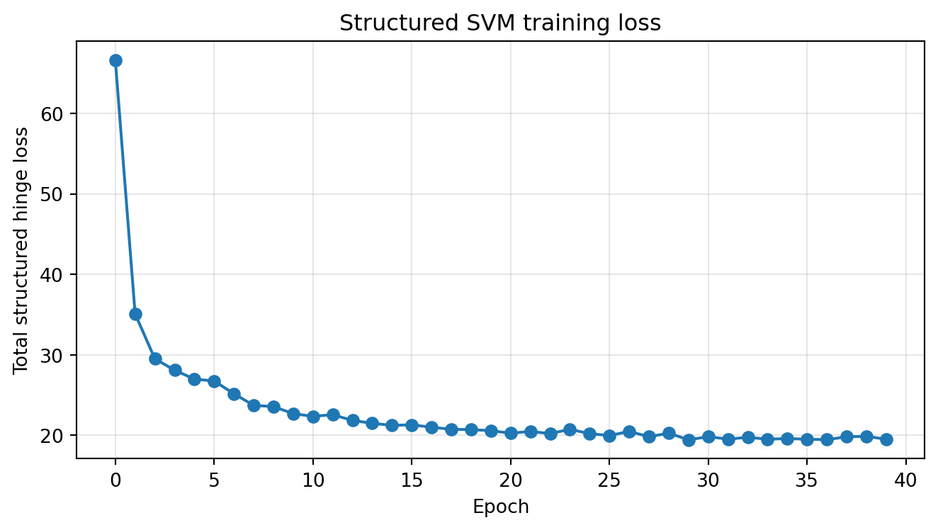
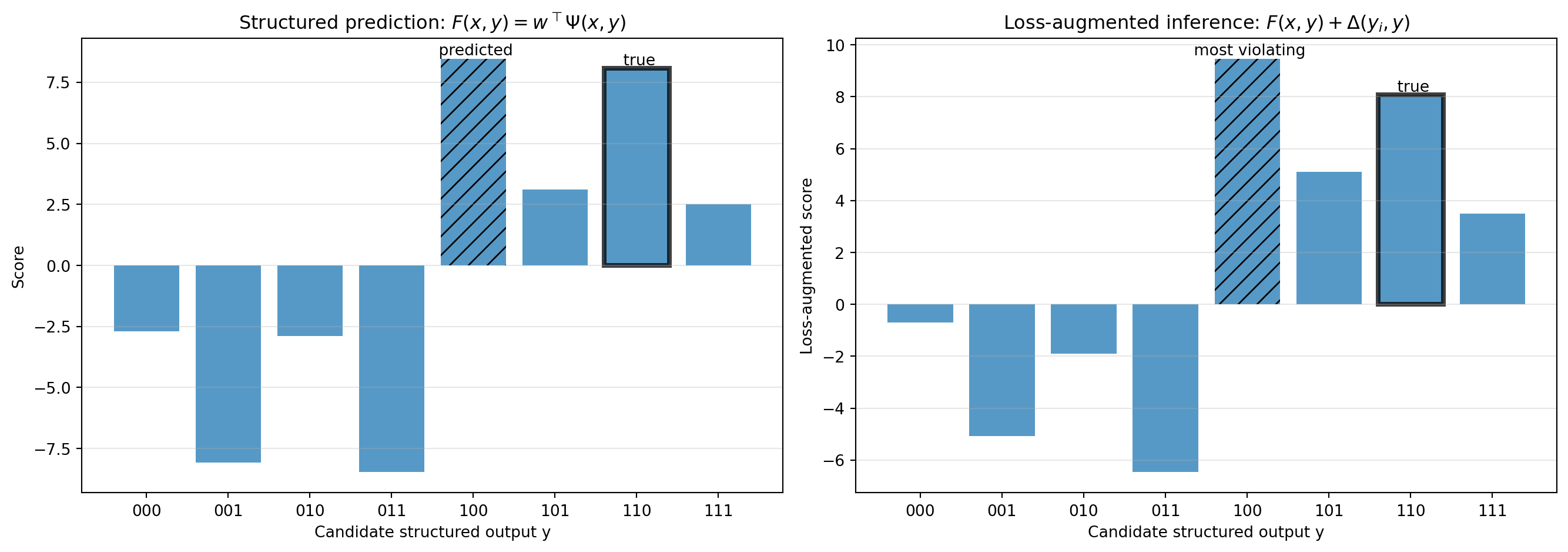
A structured SVM uses a joint feature map \(\Psi (x, y)\) and a scoring function \(F(x, y) = w^\top \Psi(x, y)\). Prediction then is

\[ \hat y (x) = \arg\max_{y\in \mathcal Y}w^\top\Psi(x, y) \]

The margin constraints become

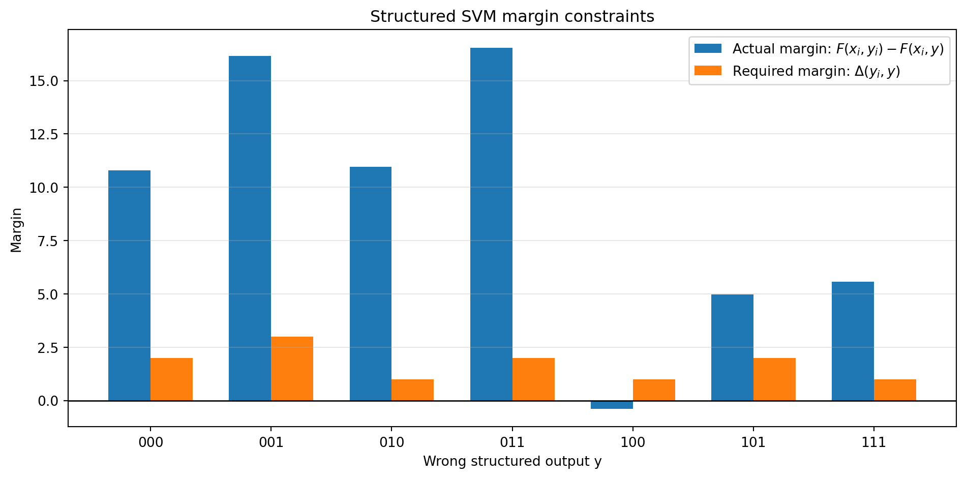
\[ w^\top \Psi(x_i, y_i) - w^\top \Psi (x_i, y)\geq \Delta(y_i, y)- \xi_i \quad \forall y\neq y_i \]

Here \(\Delta(y_i, y)\) is a task-specific loss measuring how wrong prediction \(y\) is compared with the true structured output \(y_i\).

Structured SVM generalizes the maximum-margin principle from class labels to structured prediction.

import numpy as np
import matplotlib.pyplot as plt

from itertools import product

L = 3          # sequence length
K = 2          # number of possible tags: 0 or 1
d = 2          # number of features per token

# All possible structured outputs y
# Example: (0, 1, 1)
Y_space = list(product(range(K), repeat=L))

print("Structured output space:")
for y in Y_space:
    print(y)
    
def psi(x, y):
    """
    Joint feature map Psi(x, y).

    x has shape: (L, d)
    y is a tuple of length L, such as (0, 1, 1)

    Output feature vector contains:
        - emission features
        - transition features
    """

    # Emission part: K labels, each with d features
    emission = np.zeros(K * d)

    for t in range(L):
        label = y[t]
        start = label * d
        end = start + d
        emission[start:end] += x[t]

    # Transition part: K x K possible transitions
    transition = np.zeros(K * K)

    for t in range(L - 1):
        prev_label = y[t]
        next_label = y[t + 1]
        transition_index = prev_label * K + next_label
        transition[transition_index] += 1

    return np.concatenate([emission, transition])
    
def score(w, x, y):
    return w @ psi(x, y)


def predict(w, x):
    """
    Standard structured prediction:
    choose y with largest score F(x, y).
    """
    scores = [score(w, x, y) for y in Y_space]
    best_index = np.argmax(scores)
    return Y_space[best_index]


def hamming_loss(y_true, y_pred):
    """
    Task-specific structured loss Delta(y_true, y_pred).

    Here we use Hamming loss:
    number of positions where the predicted sequence differs.
    """
    return sum(a != b for a, b in zip(y_true, y_pred))


def loss_augmented_predict(w, x, y_true):
    """
    Loss-augmented inference:

    argmax_y [F(x, y) + Delta(y_true, y)]

    This finds the most violating incorrect structure.
    """
    values = [
        score(w, x, y) + hamming_loss(y_true, y)
        for y in Y_space
    ]

    best_index = np.argmax(values)
    return Y_space[best_index]

Structured output space:
(0, 0, 0)
(0, 0, 1)
(0, 1, 0)
(0, 1, 1)
(1, 0, 0)
(1, 0, 1)
(1, 1, 0)
(1, 1, 1)

np.random.seed(7)

n_samples = 80

X_train = []
Y_train = []

for i in range(n_samples):
    x = np.random.randn(L, d)

    # Simple hidden rule:
    # if first feature is positive, label is 1;
    # otherwise label is 0.
    y = tuple((x[:, 0] > 0).astype(int))

    X_train.append(x)
    Y_train.append(y)

X_train = np.array(X_train)

print("Example input x:")
print(X_train[0])

print("\nTrue structured output y:")
print(Y_train[0])


feature_dim = K * d + K * K
w = np.zeros(feature_dim)

learning_rate = 0.05
regularization = 0.01
epochs = 40

loss_history = []

for epoch in range(epochs):
    total_loss = 0

    for x_i, y_i in zip(X_train, Y_train):

        # Find most violating structured output
        y_hat = loss_augmented_predict(w, x_i, y_i)

        true_score = score(w, x_i, y_i)
        wrong_score = score(w, x_i, y_hat)
        delta = hamming_loss(y_i, y_hat)

        violation = wrong_score + delta - true_score

        # Regularization shrinkage
        w = (1 - learning_rate * regularization) * w

        # Structured hinge update
        if violation > 0:
            w += learning_rate * (psi(x_i, y_i) - psi(x_i, y_hat))
            total_loss += violation

    loss_history.append(total_loss)

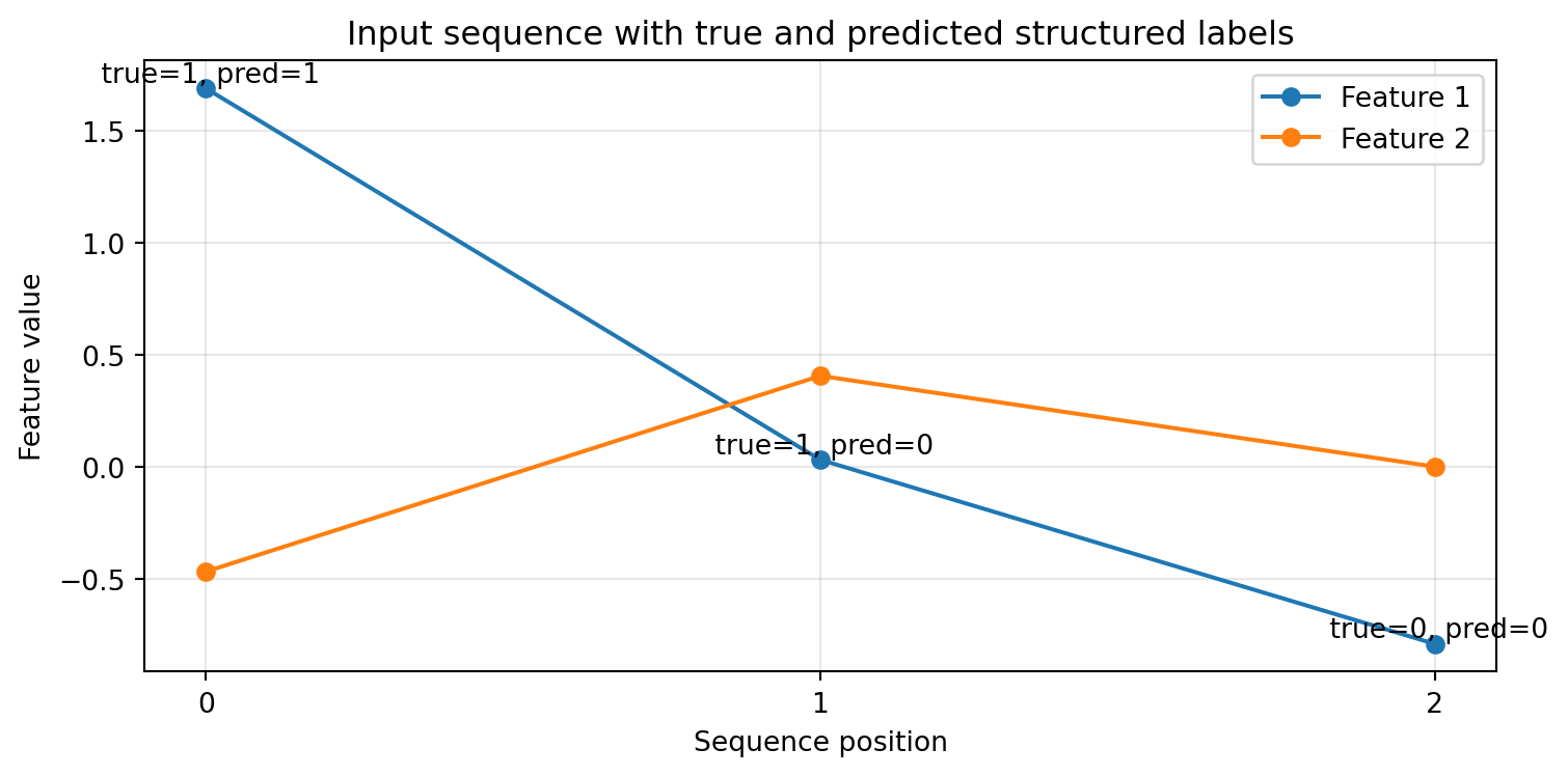
Example input x:
[[ 1.6905257  -0.46593737]
 [ 0.03282016  0.40751628]
 [-0.78892303  0.00206557]]

True structured output y:
(np.int64(1), np.int64(1), np.int64(0))

plt.figure(figsize=(7, 4))

plt.plot(loss_history, marker="o")

plt.title("Structured SVM training loss")
plt.xlabel("Epoch")
plt.ylabel("Total structured hinge loss")
plt.grid(alpha=0.3)

plt.tight_layout()
plt.show()

sample_index = 0

x_test = X_train[sample_index]
y_true = Y_train[sample_index]
y_pred = predict(w, x_test)
y_violating = loss_augmented_predict(w, x_test, y_true)

labels = ["".join(map(str, y)) for y in Y_space]

scores = np.array([
    score(w, x_test, y)
    for y in Y_space
])

loss_augmented_scores = np.array([
    score(w, x_test, y) + hamming_loss(y_true, y)
    for y in Y_space
])

true_index = Y_space.index(y_true)
pred_index = Y_space.index(y_pred)
violating_index = Y_space.index(y_violating)

print("True output:      ", y_true)
print("Predicted output: ", y_pred)
print("Most violating y: ", y_violating)

True output:       (np.int64(1), np.int64(1), np.int64(0))
Predicted output:  (1, 0, 0)
Most violating y:  (1, 0, 0)

fig, axes = plt.subplots(1, 2, figsize=(14, 5))

ax = axes[0]

bars = ax.bar(labels, scores, alpha=0.75)

bars[true_index].set_edgecolor("black")
bars[true_index].set_linewidth(3)

bars[pred_index].set_hatch("//")

ax.set_title(r"Structured prediction: $F(x,y)=w^\top\Psi(x,y)$")
ax.set_xlabel("Candidate structured output y")
ax.set_ylabel("Score")
ax.grid(alpha=0.3, axis="y")

ax.text(
    true_index,
    scores[true_index],
    " true",
    ha="center",
    va="bottom"
)

ax.text(
    pred_index,
    scores[pred_index],
    " predicted",
    ha="center",
    va="bottom"
)

ax = axes[1]

bars = ax.bar(labels, loss_augmented_scores, alpha=0.75)

bars[true_index].set_edgecolor("black")
bars[true_index].set_linewidth(3)

bars[violating_index].set_hatch("//")

ax.set_title(r"Loss-augmented inference: $F(x,y)+\Delta(y_i,y)$")
ax.set_xlabel("Candidate structured output y")
ax.set_ylabel("Loss-augmented score")
ax.grid(alpha=0.3, axis="y")

ax.text(
    true_index,
    loss_augmented_scores[true_index],
    " true",
    ha="center",
    va="bottom"
)

ax.text(
    violating_index,
    loss_augmented_scores[violating_index],
    " most violating",
    ha="center",
    va="bottom"
)

plt.tight_layout()
plt.show()

wrong_outputs = [y for y in Y_space if y != y_true]
wrong_labels = ["".join(map(str, y)) for y in wrong_outputs]

true_score = score(w, x_test, y_true)

actual_margins = np.array([
    true_score - score(w, x_test, y)
    for y in wrong_outputs
])

required_margins = np.array([
    hamming_loss(y_true, y)
    for y in wrong_outputs
])

plt.figure(figsize=(10, 5))

x_pos = np.arange(len(wrong_outputs))
width = 0.35

plt.bar(
    x_pos - width / 2,
    actual_margins,
    width,
    label=r"Actual margin: $F(x_i,y_i)-F(x_i,y)$"
)

plt.bar(
    x_pos + width / 2,
    required_margins,
    width,
    label=r"Required margin: $\Delta(y_i,y)$"
)

plt.axhline(0, color="black", linewidth=1)

plt.xticks(x_pos, wrong_labels)
plt.title("Structured SVM margin constraints")
plt.xlabel("Wrong structured output y")
plt.ylabel("Margin")
plt.grid(alpha=0.3, axis="y")
plt.legend()

plt.tight_layout()
plt.show()

positions = np.arange(L)

plt.figure(figsize=(8, 4))

plt.plot(
    positions,
    x_test[:, 0],
    marker="o",
    label="Feature 1"
)

plt.plot(
    positions,
    x_test[:, 1],
    marker="o",
    label="Feature 2"
)

for t in range(L):
    plt.text(
        t,
        x_test[t, 0],
        f" true={y_true[t]}, pred={y_pred[t]}",
        ha="center",
        va="bottom"
    )

plt.title("Input sequence with true and predicted structured labels")
plt.xlabel("Sequence position")
plt.ylabel("Feature value")
plt.xticks(positions)
plt.grid(alpha=0.3)
plt.legend()

plt.tight_layout()
plt.show()

9.6. Incremental and Online SVM

Classical SVM training is batch-based (the model is trained on a fixed dataset). However, real-world systems may receive data streams over time.

Incremental or online SVM methods update the model when new observations arrive. These are useful when data arrive continuously, the environment changes, retraining from scratch is expensive, and model adaption is necessary.

The main challenge is preserving the support-vector structure while updating the solution efficiently. Once deployed, a model may face changing distributions.

10. Modeling Issues

10.1. Feature Scaling

SVMs are sensitive to feature scale because the margin depends on inner products and distances. If one variable has a much larger scale than another, it can dominate the hyperplane or the kernel.

For example, if \(x_1\) is income in dollars, and \(x_2\) is age in years, then the magnitude of \(x_1\) may dominate the dot product \(x^\top z\) or the RBF distance \(\|x-z\|^2\).

Therefore, SVMs are typically used with standardization:

\[ z_j = \frac{x_j-\mu_j}{\sigma_j} \]

Scaling must be fit only on training data and then applied to validation/test data to avoid leakage.

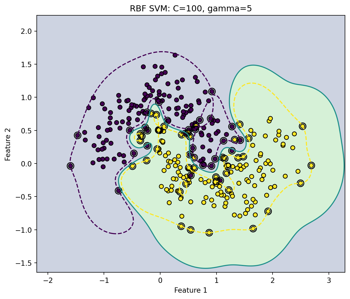
10.2. Choosing \(C\) and \(\gamma\)

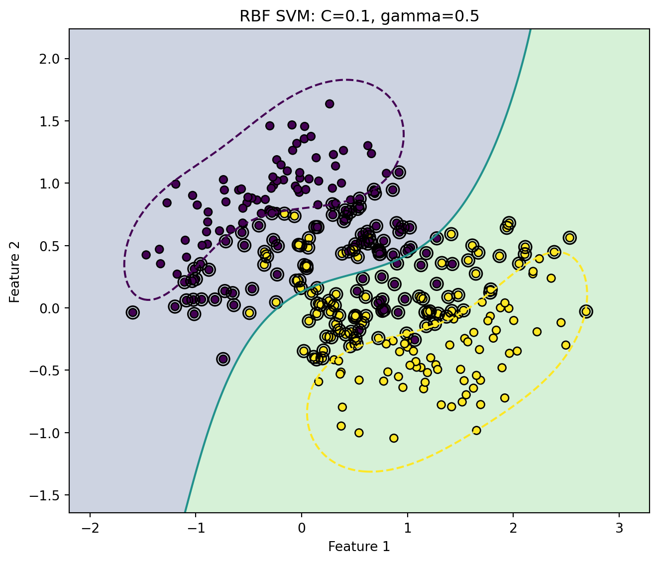
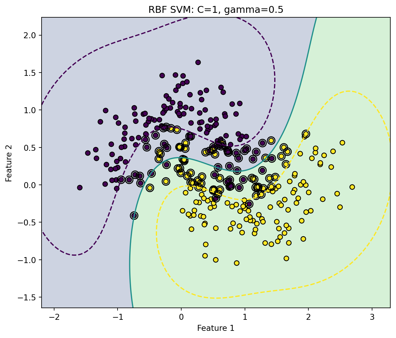
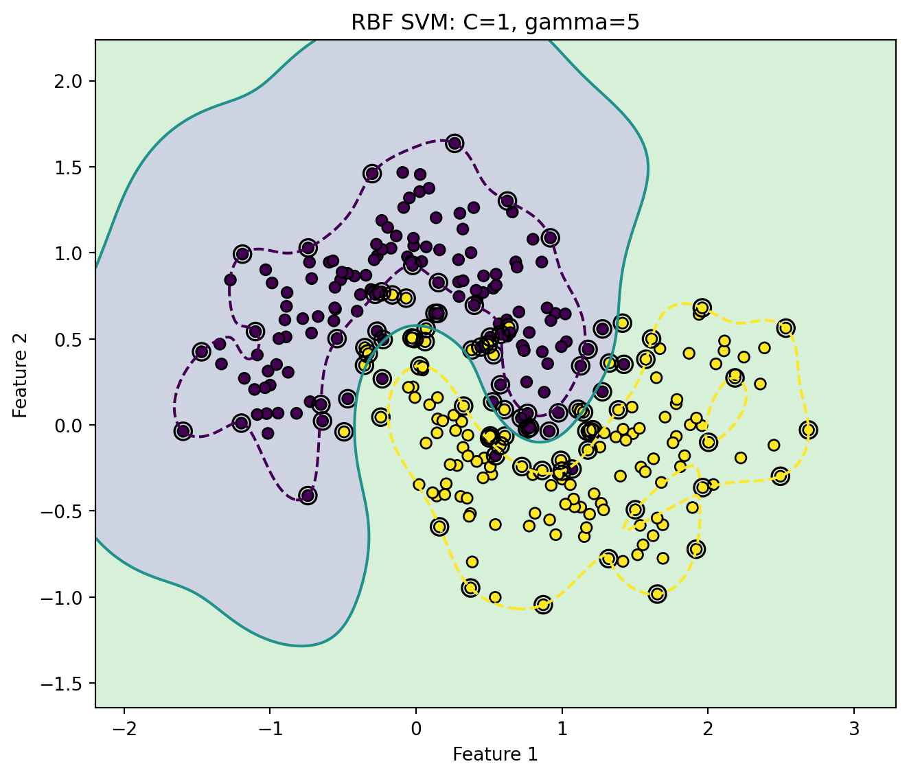
For the RBF SVM, the two most important hyperparameters are usually \(C\) and \(\gamma\).

The parameter \(C\) controls regularization:

• small \(C\): wide margin, more tolerance for errors;
• large \(C\): narrow margin, less tolerance for errors.

The parameter \(\gamma\) controls kernel locality:

• small \(\gamma\): smooth boundary;
• large \(\gamma\): highly local, flexible boundary.

Together, \(C\) and \(\gamma\) determine model complexity.

A common model-selection procedure (again) is grid search with cross-validation:

\[ (C^*, \gamma^*) =\arg\min_{C, \gamma} CV(C, \gamma) \]

For classification error,

\[ CV(C, \gamma) = \frac{1}{V} \sum_{v=1}^V \frac{1}{I_v}\sum_{i\in I_v}\mathbf{I}\{y_i\neq \hat y_{C,\gamma}^{(-v)}(x_i)\} \]

import numpy as np
import matplotlib.pyplot as plt
from sklearn.datasets import make_moons
from sklearn.svm import SVC

X, y = make_moons(n_samples=300, noise=0.25, random_state=42)
y_signed = np.where(y == 0, -1, 1)

x_min, x_max = X[:, 0].min() - 0.6, X[:, 0].max() + 0.6
y_min, y_max = X[:, 1].min() - 0.6, X[:, 1].max() + 0.6

xx, yy = np.meshgrid(
    np.linspace(x_min, x_max, 350),
    np.linspace(y_min, y_max, 350)
)

grid = np.c_[xx.ravel(), yy.ravel()]

settings = [
    (0.1, 0.5),
    (1, 0.5),
    (1, 5),
    (100, 5)
]

for C, gamma in settings:
    clf = SVC(kernel="rbf", C=C, gamma=gamma)
    clf.fit(X, y_signed)

    Z = clf.decision_function(grid).reshape(xx.shape)

    plt.figure(figsize=(7, 6))
    plt.contourf(xx, yy, Z > 0, alpha=0.25)
    plt.contour(xx, yy, Z, levels=[-1, 0, 1], linestyles=["--", "-", "--"])
    plt.scatter(X[:, 0], X[:, 1], c=y_signed, edgecolor="k", s=35)
    plt.scatter(
        clf.support_vectors_[:, 0],
        clf.support_vectors_[:, 1],
        s=90,
        facecolors="none",
        edgecolors="k",
        linewidths=1.2
    )
    plt.title(f"RBF SVM: C={C}, gamma={gamma}")
    plt.xlabel("Feature 1")
    plt.ylabel("Feature 2")
    plt.tight_layout()
    plt.show()

10.3. Computational Complexity

Kernel SVMs require operations involving the kernel matrix \(K\in \mathbb R^{n\times n}\). This can be expensive for large \(n\), because the matrix has \(n^2\) entries. Storage may require \(O(n^2)\) memory, and training can be computationally expensive depending on the solver and problem structure.

Linear SVMs are often preferred for very large sparse datasets such as text classification because they avoid full kernel matrix and scale better.

11. Examples

11.1. Breast Cancer Classification

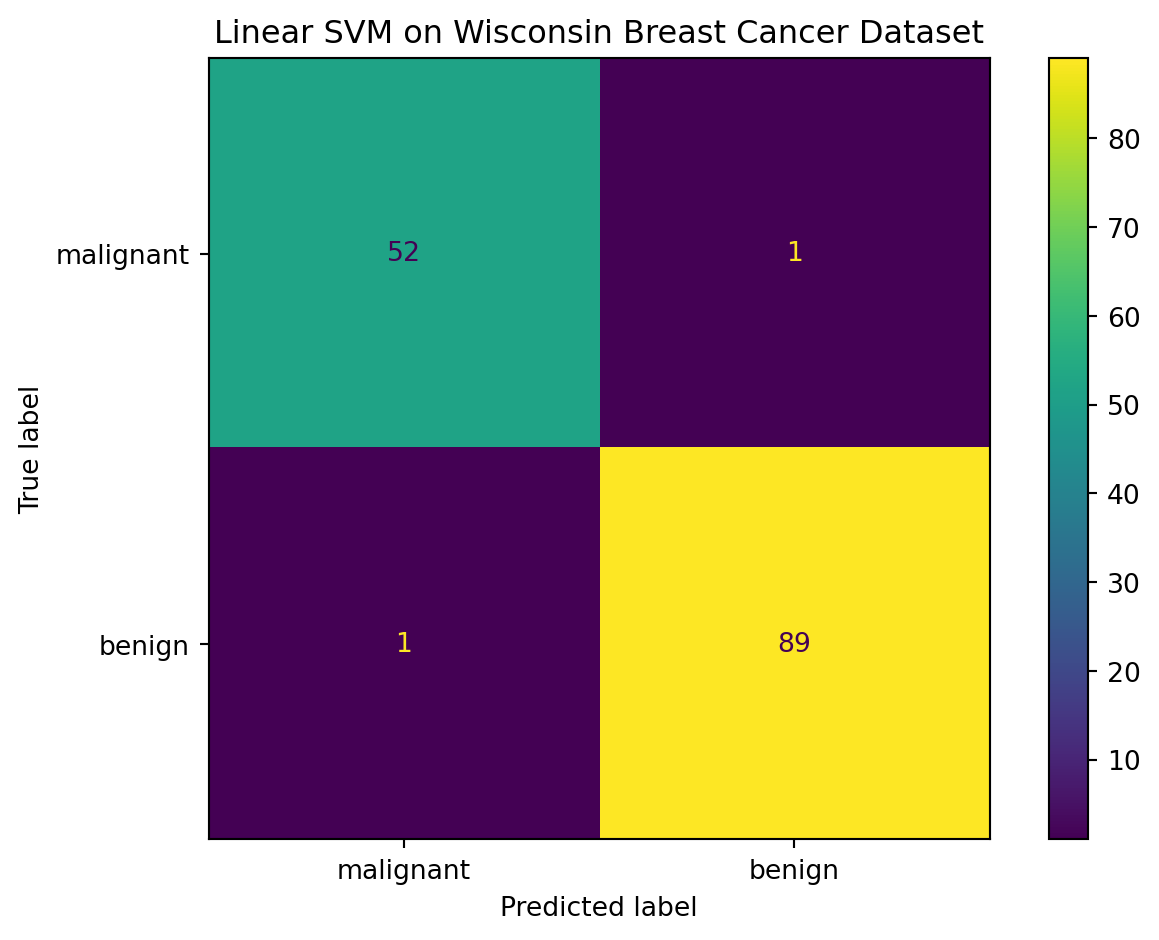
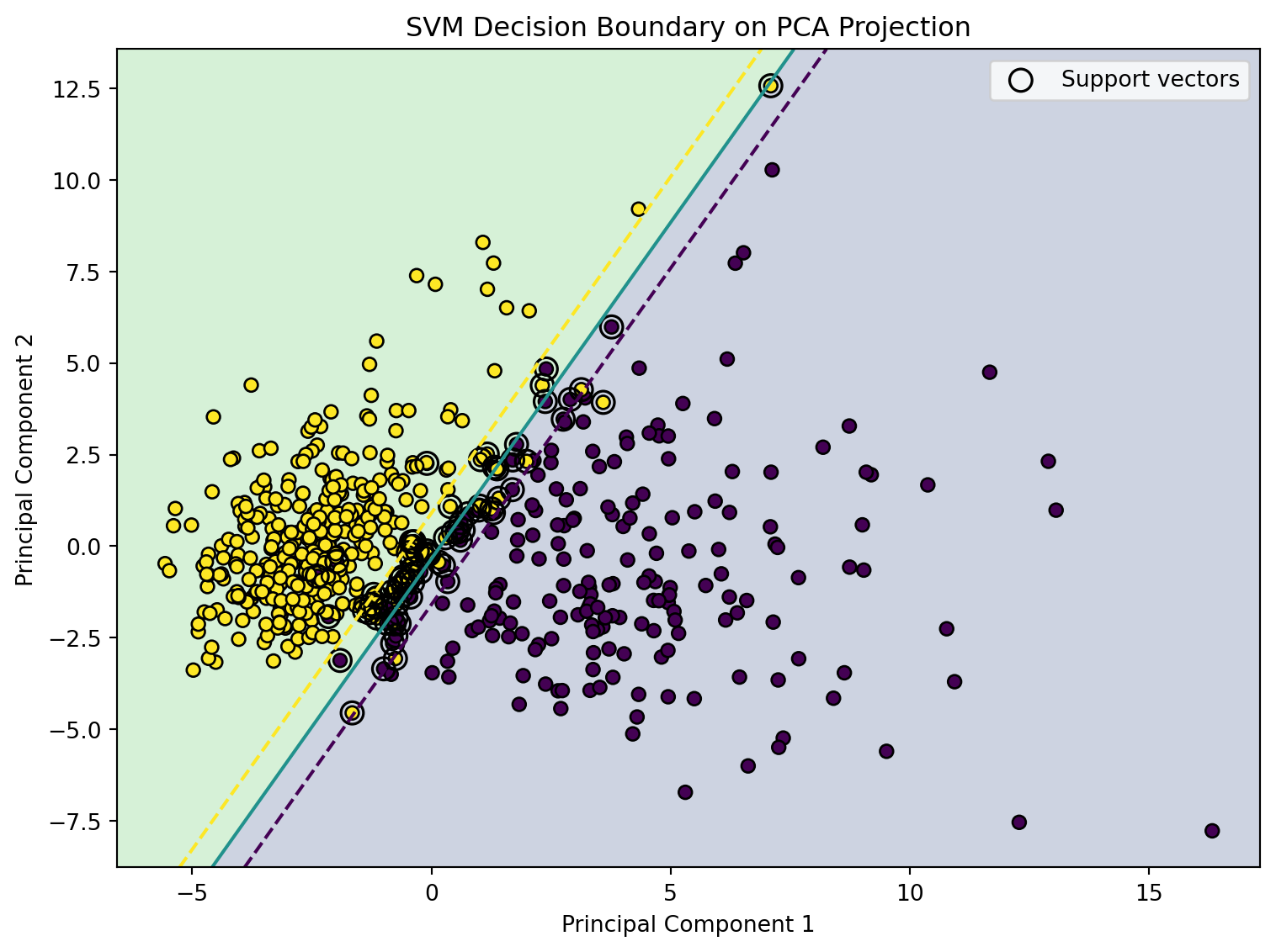
The Wisconsin breast cancer dataset is a common real dataset for binary classification. Each observation describes features computed from a digitized image of a breast mass, and the target indicates malignant or benign diagnosis.

import numpy as np
import matplotlib.pyplot as plt
from sklearn.datasets import load_breast_cancer
from sklearn.pipeline import Pipeline
from sklearn.preprocessing import StandardScaler
from sklearn.svm import SVC
from sklearn.decomposition import PCA
from sklearn.model_selection import train_test_split
from sklearn.metrics import ConfusionMatrixDisplay, classification_report

data = load_breast_cancer()

X = data.data
y = data.target

X_train, X_test, y_train, y_test = train_test_split(
    X, y,
    test_size=0.25,
    random_state=42,
    stratify=y
)

model = Pipeline([
    ("scaler", StandardScaler()),
    ("svm", SVC(kernel="linear", C=1))
])

model.fit(X_train, y_train)

print(classification_report(y_test, model.predict(X_test), target_names=data.target_names))

ConfusionMatrixDisplay.from_estimator(
    model,
    X_test,
    y_test,
    display_labels=data.target_names
)
plt.title("Linear SVM on Wisconsin Breast Cancer Dataset")
plt.tight_layout()
plt.show()

# PCA visualization
pca = PCA(n_components=2)
X_scaled = StandardScaler().fit_transform(X)
X_pca = pca.fit_transform(X_scaled)

svm_2d = SVC(kernel="linear", C=1)
svm_2d.fit(X_pca, y)

x_min, x_max = X_pca[:, 0].min() - 1, X_pca[:, 0].max() + 1
y_min, y_max = X_pca[:, 1].min() - 1, X_pca[:, 1].max() + 1

xx, yy = np.meshgrid(
    np.linspace(x_min, x_max, 400),
    np.linspace(y_min, y_max, 400)
)

grid = np.c_[xx.ravel(), yy.ravel()]
Z = svm_2d.decision_function(grid).reshape(xx.shape)

plt.figure(figsize=(8, 6))
plt.contourf(xx, yy, Z > 0, alpha=0.25)
plt.contour(xx, yy, Z, levels=[-1, 0, 1], linestyles=["--", "-", "--"])
plt.scatter(X_pca[:, 0], X_pca[:, 1], c=y, edgecolor="k", s=35)
plt.scatter(
    svm_2d.support_vectors_[:, 0],
    svm_2d.support_vectors_[:, 1],
    s=100,
    facecolors="none",
    edgecolors="k",
    linewidths=1.2,
    label="Support vectors"
)
plt.title("SVM Decision Boundary on PCA Projection")
plt.xlabel("Principal Component 1")
plt.ylabel("Principal Component 2")
plt.legend()
plt.tight_layout()
plt.show()

              precision    recall  f1-score   support

   malignant       0.98      0.98      0.98        53
      benign       0.99      0.99      0.99        90

    accuracy                           0.99       143
   macro avg       0.99      0.99      0.99       143
weighted avg       0.99      0.99      0.99       143

This example shows two things:

1. In the full feature space, the SVM is trained on all available diagnostic variables.
2. In the PCA plot, we can visualize the separating boundary approximately in two dimensions.

11.2. Handwritten Digit Recognition

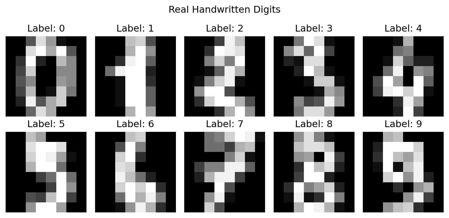
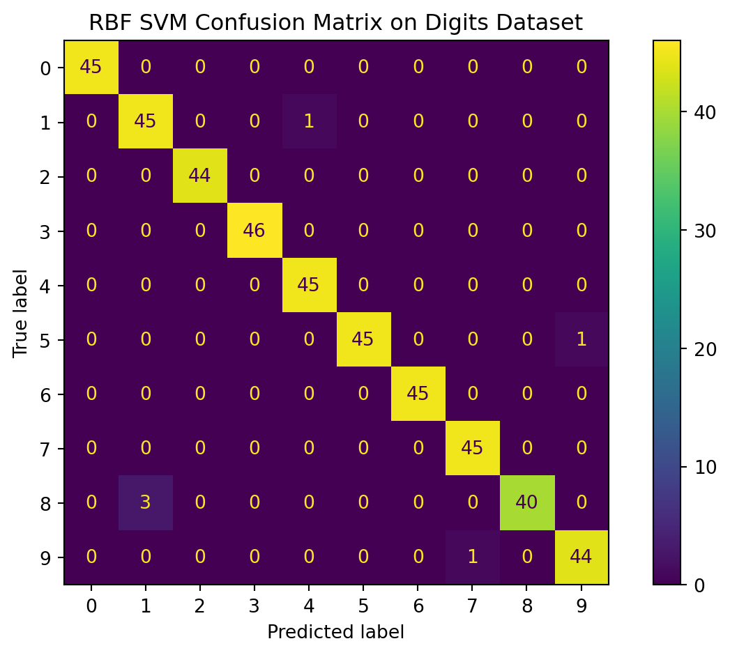
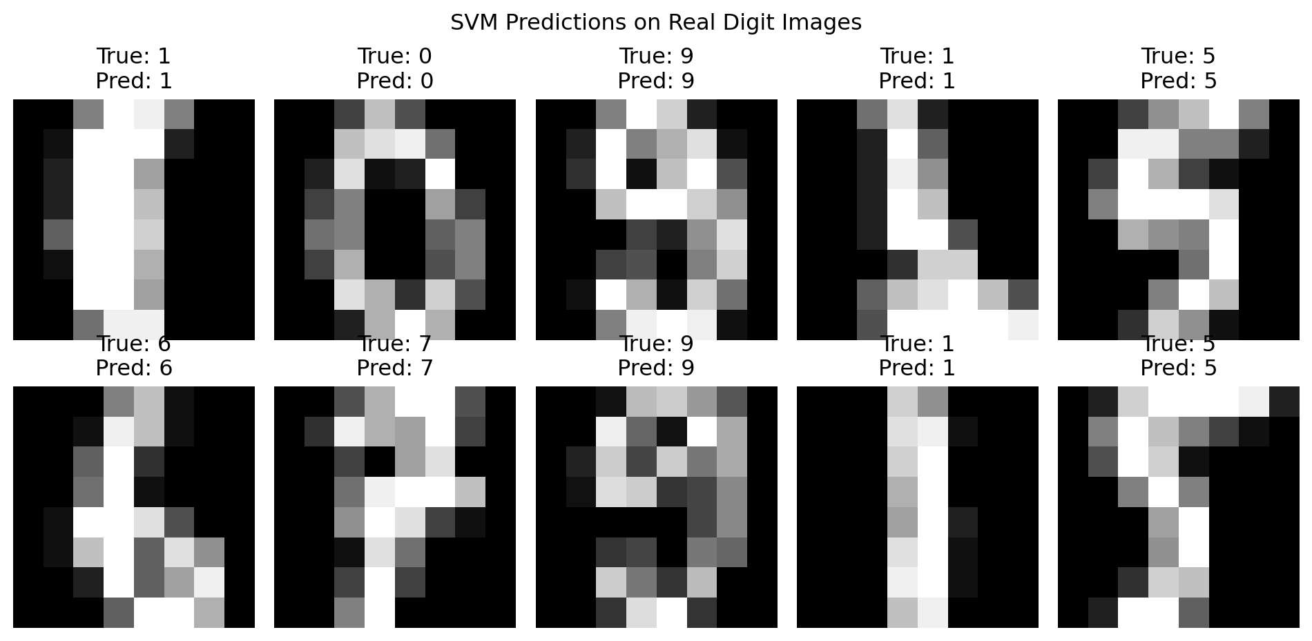
SVMs have historically been used in handwritten digit recognition, including postal ZIP code recognition. In this setting, each image is represented as a vector of pixel intensities.

The scikit-learn digits dataset contains \(8\times 8\) grayscale digit images. Each image is flattened into \(x_i\in \mathbb R^{64}\). The label is \(y_i\in \{0,1 ,\dots, 9\}\). A multiclass SVM can classify the digits.

import numpy as np
import matplotlib.pyplot as plt
from sklearn.datasets import load_digits
from sklearn.pipeline import Pipeline
from sklearn.preprocessing import StandardScaler
from sklearn.svm import SVC
from sklearn.model_selection import train_test_split
from sklearn.metrics import ConfusionMatrixDisplay, accuracy_score

digits = load_digits()

X = digits.data
y = digits.target
images = digits.images

# Display real digit images
plt.figure(figsize=(8, 4))
for i in range(10):
    plt.subplot(2, 5, i + 1)
    plt.imshow(images[i], cmap="gray")
    plt.title(f"Label: {y[i]}")
    plt.axis("off")
plt.suptitle("Real Handwritten Digits")
plt.tight_layout()
plt.show()

X_train, X_test, y_train, y_test, images_train, images_test = train_test_split(
    X, y, images,
    test_size=0.25,
    random_state=42,
    stratify=y
)

model = Pipeline([
    ("scaler", StandardScaler()),
    ("svm", SVC(kernel="rbf", C=10, gamma=0.001))
])

model.fit(X_train, y_train)
y_pred = model.predict(X_test)

print("Test accuracy:", accuracy_score(y_test, y_pred))

ConfusionMatrixDisplay.from_predictions(y_test, y_pred)
plt.title("RBF SVM Confusion Matrix on Digits Dataset")
plt.tight_layout()
plt.show()

# Display a few predictions
plt.figure(figsize=(10, 5))
for i in range(10):
    plt.subplot(2, 5, i + 1)
    plt.imshow(images_test[i], cmap="gray")
    plt.title(f"True: {y_test[i]}\nPred: {y_pred[i]}")
    plt.axis("off")
plt.suptitle("SVM Predictions on Real Digit Images")
plt.tight_layout()
plt.show()

Test accuracy: 0.9866666666666667

11.3. Text Classification

SVMs have been widely used in text classification because text data are often high-dimensional and sparse. A document can be represented by a term-frequency or TF-IDF vector:

\[ x_i = (x_{i1}, x_{i2}, \dots, x_{ip}) \]

where \(p\) may be thousands or tens of thousands of vocabulary terms.

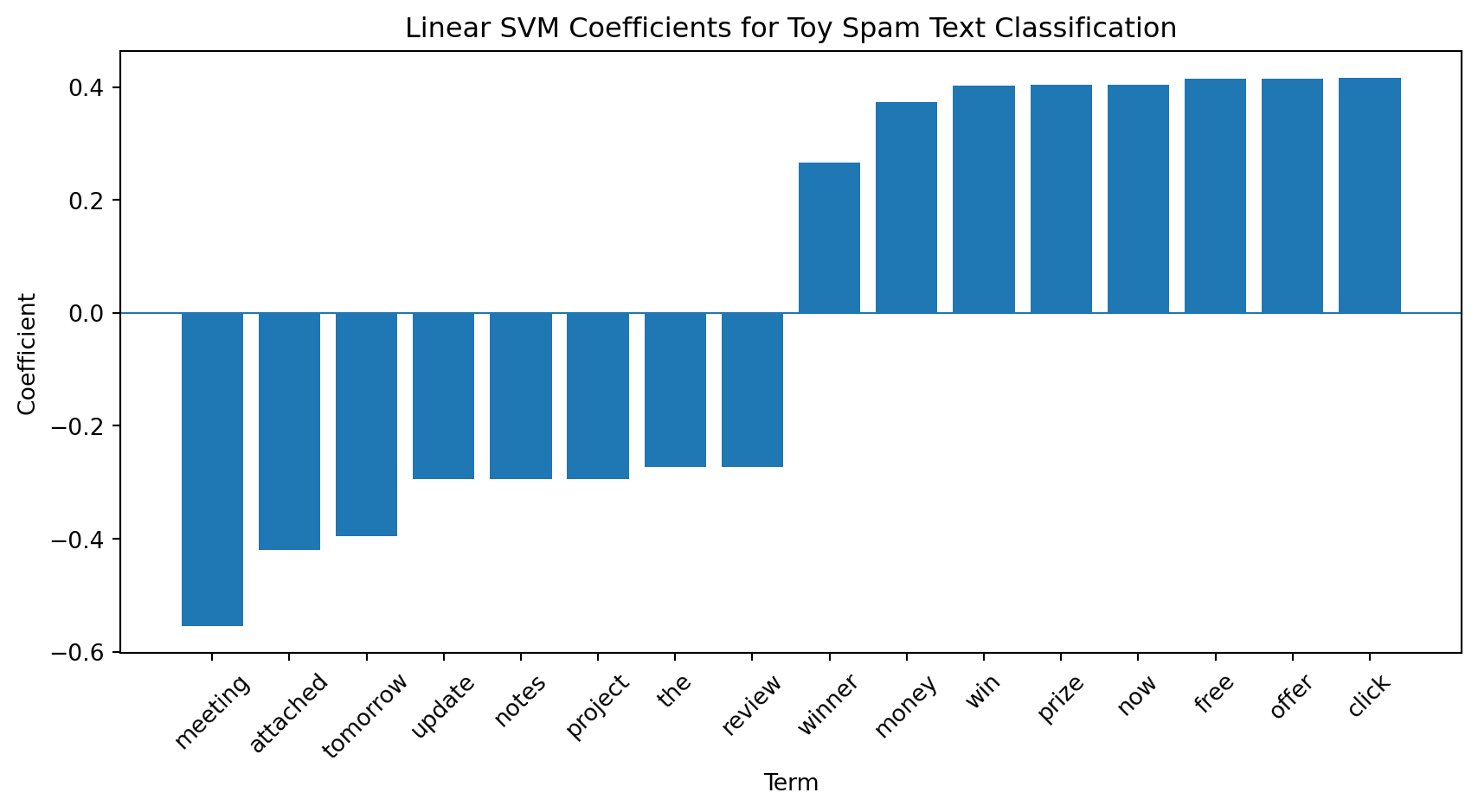
A linear SVM is often enough because high-dimensional sparse text data may sometimes become approximately linearly separable.

For binary spam detection, labels may be

\[ y_i = \begin{cases}+1, & \text{spam}, \\ -1, & \text{not spam}\end{cases} \]

The classifier is

\[ \hat y(x) = \text{sign} (w^\top x+ b) \]

Terms with large positive coefficients contribute toward the spam class, while terms with large negative coefficients contribute toward the non-spam class.

import numpy as np
import matplotlib.pyplot as plt
from sklearn.feature_extraction.text import TfidfVectorizer
from sklearn.svm import LinearSVC

documents = [
    "win money now claim your prize",
    "urgent prize winner click now",
    "free money offer click link",
    "meeting schedule attached tomorrow",
    "project update meeting notes",
    "please review the attached report",
    "limited offer win free cash",
    "team meeting agenda for tomorrow"
]

labels = np.array([1, 1, 1, -1, -1, -1, 1, -1])

vectorizer = TfidfVectorizer()
X = vectorizer.fit_transform(documents)

clf = LinearSVC(C=1)
clf.fit(X, labels)

terms = np.array(vectorizer.get_feature_names_out())
coefs = clf.coef_[0]

top_positive = np.argsort(coefs)[-8:]
top_negative = np.argsort(coefs)[:8]

selected_terms = np.concatenate([top_negative, top_positive])
selected_coefs = coefs[selected_terms]

plt.figure(figsize=(9, 5))
plt.bar(terms[selected_terms], selected_coefs)
plt.axhline(0, linewidth=0.8)
plt.title("Linear SVM Coefficients for Toy Spam Text Classification")
plt.xlabel("Term")
plt.ylabel("Coefficient")
plt.xticks(rotation=45)
plt.tight_layout()
plt.show()

---

Support Vector Machines are maximum-margin learning methods grounded in statistical learning theory and convex optimization. Their central idea is that good classification should not merely separate training data but separate them with the widest possible margin.

For linearly separable data, the hard-margin SVM finds the hyperplane maximizing

\[ \frac{2}{\|w\|}. \]

For nonseparable data, the soft-margin SVM introduces slack variables and balances margin width against violations through the parameter C. Through the hinge loss, SVMs become regularized empirical risk minimizers that penalize points inside the margin or on the wrong side of the boundary.

The dual formulation reveals the sparse structure of the model: predictions depend only on support vectors. The kernel trick extends SVMs to nonlinear classification by replacing inner products with kernel functions, allowing linear separation in implicit high-dimensional feature spaces. This makes SVMs powerful for nonlinear boundaries, high-dimensional data, text classification, bioinformatics, image recognition, medicine, finance, and anomaly detection.

SVMs also extend beyond binary classification. SVR uses an \(\epsilon\)-insensitive tube for regression. Multiclass SVMs combine binary classifiers. \(\nu\)-SVM provides an alternative parameterization. One-class SVM estimates the support of a distribution for novelty detection. Structured SVM generalizes maximum-margin learning to complex outputs.

Next chapter: Data modeling - ANN

Footnotes

1. Since \(1-y_i(w^\top x_i+b)\leq 0\), \(\sum_{i=1}^n \lambda_i [1-y_i(w^\top x_i+b)]\leq 0\), so \(\mathcal L(w,b,\lambda) = \frac{1}{2}||w||_2 + \sum_{i=1}^n \lambda_i [1-y_i(w^\top x_i+b)]\leq \frac{1}{2}||w||_2\). That means the Lagrangian gives a lower bound on the primal objective.